Fundamentals of predictive modeling
DataRobot offers both generative and predictive AI solutions.
Predicitve AI, available in both the Classic and NextGen experiences, uses automated machine learning (AutoML) to build models that solve real-world problems across domains and industries. DataRobot takes the data you provide, generates multiple machine learning (ML) models, and recommends the best model to put into use. You don't need to be a data scientist to build ML models using DataRobot, but an understanding of the basics will help you build better models. Your domain knowledge and DataRobot's AI expertise will lead to successful models that solve problems with speed and accuracy.
DataRobot supports many different approaches to ML modeling—supervised learning, unsupervised learning, time series modeling, segmented modeling, multimodal modeling, and more. This section describes these approaches and also provides tips for analyzing and selecting the best models for deployment.
Generative AI (GenAI), available in DataRobot's NextGen Workbench, allows you to build, govern, and operate enterprise-grade generative AI solutions with confidence. The solution provides the freedom to rapidly innovate and adapt with the best-of-breed components of your choice (LLMs, vector databases, embedding models), across cloud environments. DataRobot's GenAI:
- Safeguards proprietary data by extending your LLMs and monitoring cost of your generative AI experiments in real-time.
- Sheppards you through creating, deploying, and maintaining safe, high-quality, generative AI applications and solutions in production.
- Lets you quickly detect and prevent unexpected and unwanted behaviors.
This section describes DataRobot's predictive solutions; see the section on GenAI for the full documentation on working with generative-related tools and options.
Predictive modeling methods
Login methods
If your organization is using an external account management system for single sign-on:
- If using LDAP, note that your username is not necessarily your registered email address. Contact your DataRobot administrator to obtain your username, if necessary.
- If using a SAML-based system, on the login page, ignore the entry box for credentials. Instead, click Single Sign-On and enter credentials on the resulting page.
ML modeling is the process of developing algorithms that learn by example from historical data. These algorithms predict outcomes and uncover patterns not easily discerned. DataRobot supports a variety of modeling methods, each suiting a specific type of data and problem type.
Supervised and unsupervised learning
The most basic form of machine learning is supervised learning.
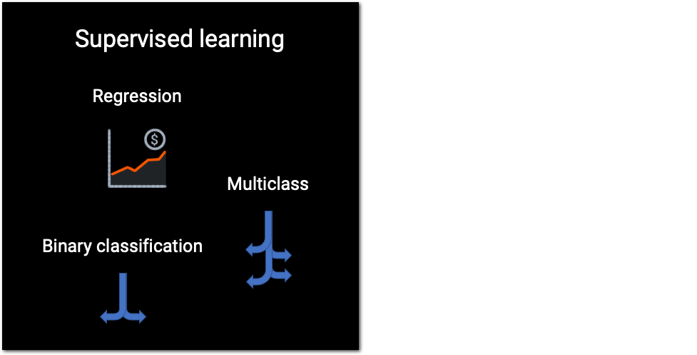
With supervised learning, you provide "labeled" data. A label in a dataset provides information to help the algorithm learn from the data. The label—also called the target—is what you're trying to predict.
-
In a regression experiment, the target is a numeric value. A regression model estimates a continuous dependent variable given a list of input variables (also referred to as features or columns). Examples of regression problems include financial forecasting, time series forecasting, maintenance scheduling, and weather analysis.
-
In a classification experiment, the target is a category. A classification model groups observations into categories by identifying shared characteristics of certain classes. It compares those characteristics to the data you're classifying and estimates how likely it is that the observation belongs to a particular class. Classification experiments can be binary (two classes) or multiclass (three or more classes). For classification, DataRobot also supports multilabel modeling where the target feature has a variable number of classes or labels; each row of the dataset is associated with one, several, or zero labels.
Another form of machine learning is unsupervised learning.

With unsupervised learning, the dataset is unlabeled and the algorithm must infer patterns in the data.
-
In an anomaly detection experiment, the algorithm detects unusual data points in your dataset. Potential uses include the detection of fraudulent transactions, faults in hardware, and human error during data entry.
-
In a clustering experiment, the algorithm splits the dataset into groups according to similarity. Clustering is useful for gaining intuition about your data. The clusters can also help label your data so that you can then use a supervised learning method on the dataset.
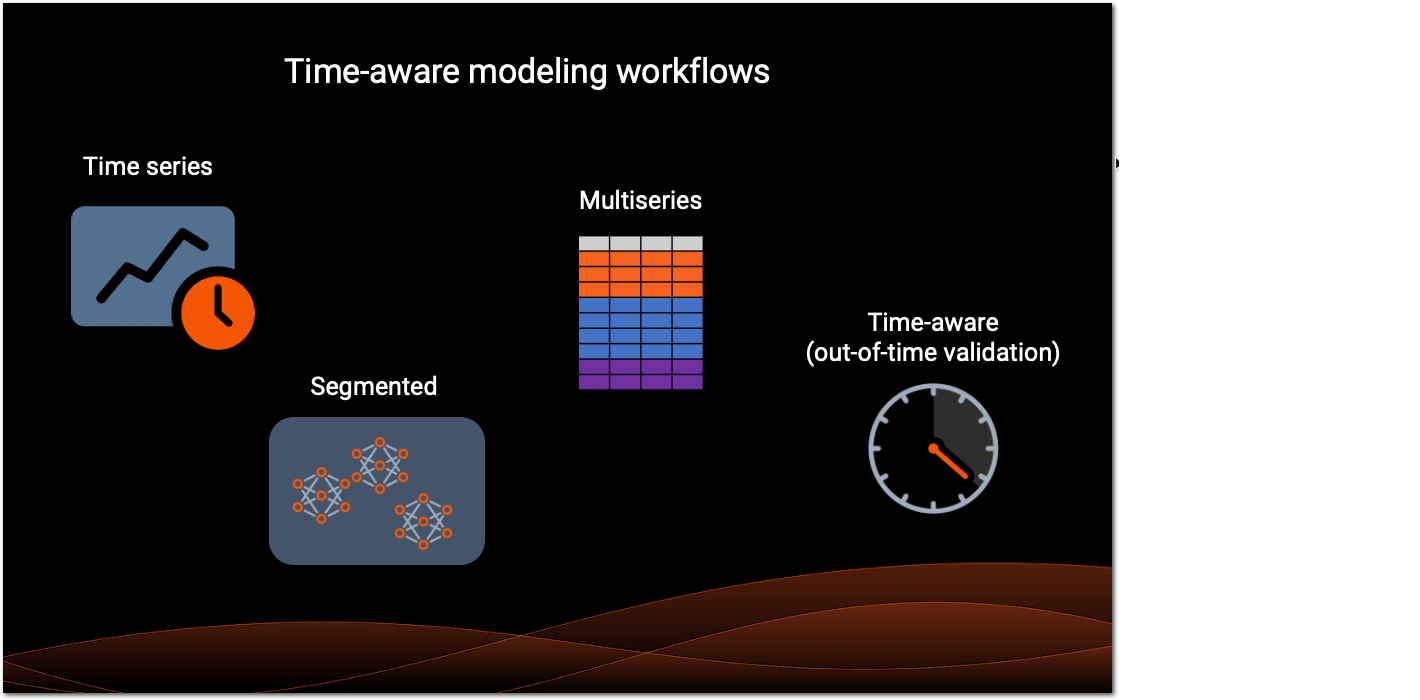
Time-aware modeling
Time data is a crucial component in solving prediction and forecasting problems. Models using time-relevant data make row-by-row predictions, time series forecasts, or current value predictions ("nowcasts"). An experiment becomes time-aware when, if the data is appropriate, the partitioning method is set to date/time.
-
With time series modeling, you can generate a forecast—a series of predictions for a period of time in the future. You train time series models on past data to predict future events. Predict a range of values in the future or use nowcasting to make a prediction at the current point in time. Use cases for time series modeling include predicting pricing and demand in domains such as finance, healthcare, and retail— basically, any domain where problems have a time component.
-
You can use time series modeling for a dataset containing a single series, but you can also build a model for a dataset that contains multiple series. For this type of multiseries experiment, one feature serves as the series identifier. An example is a "store location" identifier that essentially divides the dataset into multiple series, one for each location. So you might have four store locations (Paris, Milan, Dubai, and Tokyo) and therefore four series for modeling.
-
With a multiseries experiment, you can choose to generate a model for each series using segmented modeling. In this case, DataRobot creates a deployment using the best model for each segment.
-
Sometimes, the dataset for the problem you're solving contains date and time information, but instead of generating a forecast as you do with time series modeling, you predict a target value on each individual row. This approach is called out-of-time validation (OTV).
See What is time-aware modeling for an in-depth discussion of these strategies.
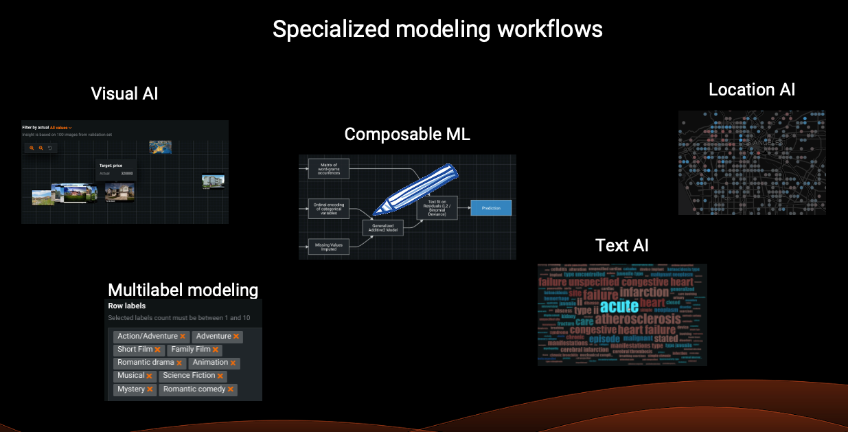
Specialized modeling workflows
DataRobot provides specialized workflows to help you address a wide range of problems.
-
Visual AI (Classic only) allows you to include images as features in your datasets. Use the image data alongside other data types to improve outcomes for various types of modeling experiments—regression, classification, anomaly detection, clustering, and more.
-
With editable blueprints, you can build and edit your own ML blueprints, incorporating DataRobot preprocessing and modeling algorithms, as well as your own models.
-
For text features in your data, use Text AI insights like Word Clouds and Text Mining to understand the impact of the text features.
-
Location AI (Classic only) supports geospatial analysis of modeling data. Use geospatial features to gain insights and visualize data using interactive maps before and after modeling.
Workbench modeling workflow
This section walks you through the steps for implementing a DataRobot modeling experiment.
-
To begin the modeling process, import your data or wrangle your data to provide a seamless, scalable, and secure way to access and transform data for modeling.
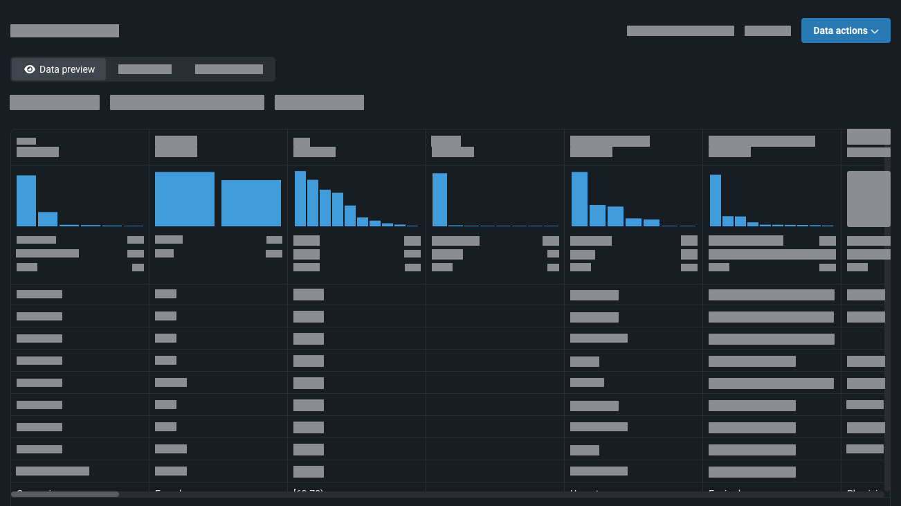
-
DataRobot conducts the first stage of exploratory data analysis, (EDA1), where it analyzes data features. When registration is complete, the Data preview tab shows feature details, including a histogram and summary statistics.
-
Next, for supervised modeling,select your target and optionally change any other basic or advanced experiment configuration settings. Then, start modeling.
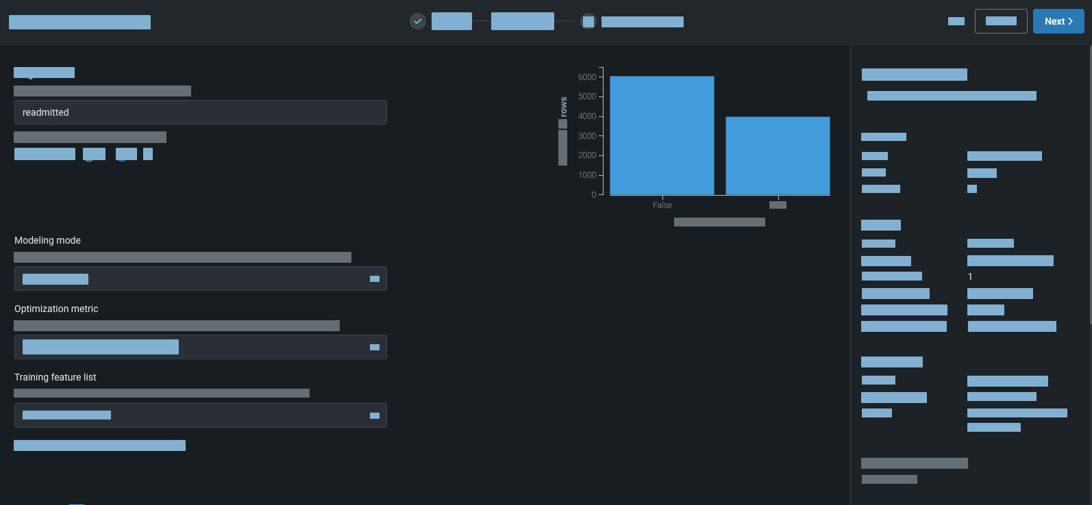
DataRobot generates feature lists from which to build models. By default, it uses the feature list with the most informative features. Alternatively, you can select different generated feature lists or create your own.
-
DataRobot further evaluates the data during EDA2, determining which features correlate to the target (feature importance) and which features are informative, among other information.
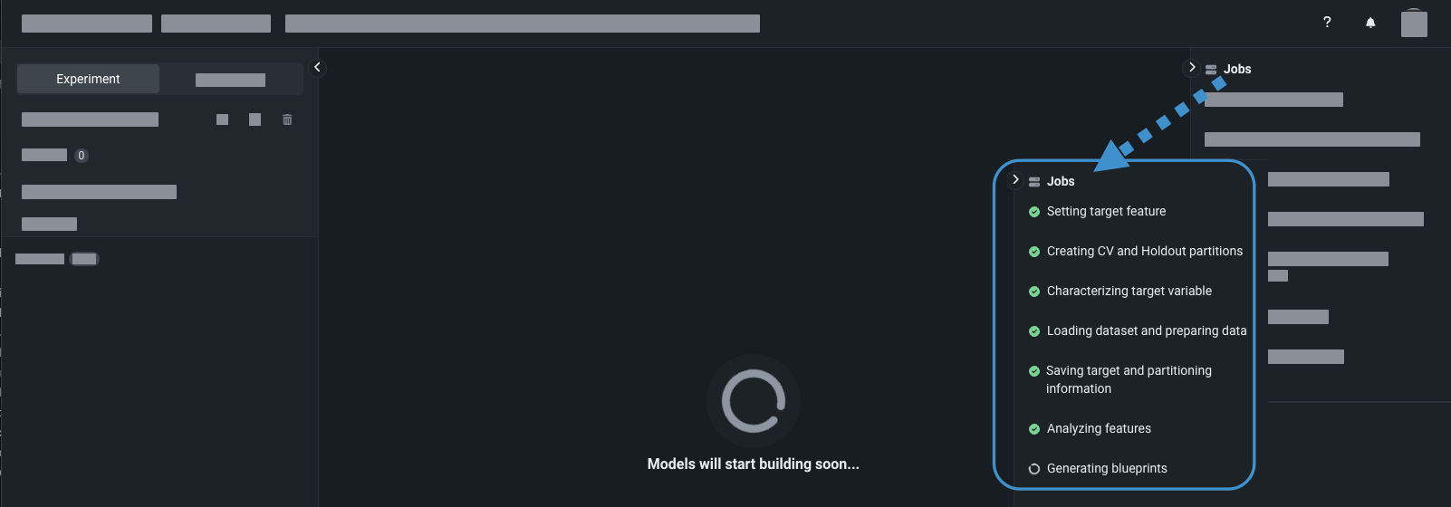
The application performs feature engineering—transforming, generating, and reducing the feature set depending on the experiment type and selected settings.
-
DataRobot selects blueprints based on the experiment type and builds candidate models.
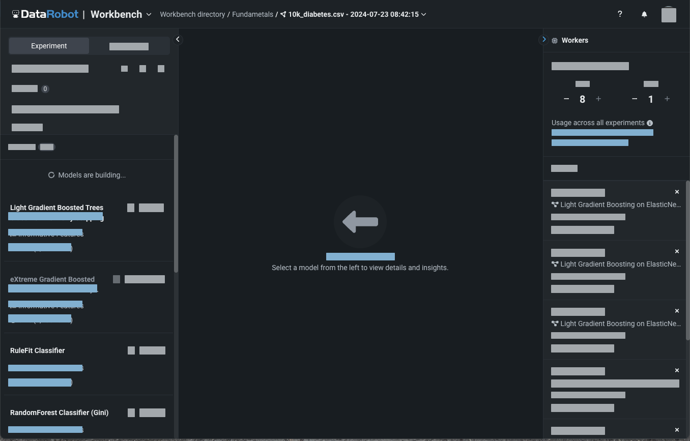
Analyze and select a model
DataRobot automatically generates models and displays them on the Leaderboard. The most accurate model is selected and trained on 100% of the data and is marked with the Prepared for Deployment badge.
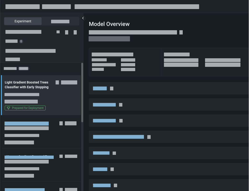
To analyze and select a model:
-
Compare models by selecting an optimization metric from the Metric dropdown.
-
Analyze the model using the visualization tools that are best suited for the type of model you are building. Use model comparison for experiments within a single Use Case.
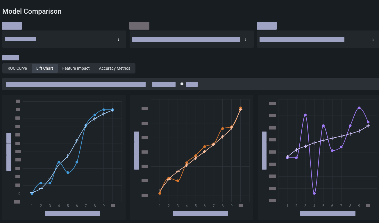
See the list of experiment types and associated visualizations below.
-
Experiment with modeling settings to potentially improve the accuracy of your model. You can try rerunning modeling using a different feature list or modeling mode.
-
After analyzing your models, select the best and send it to the Registry to create a deployment-ready model package.
Tip
It's recommended that you test predictions before deploying. If you aren't satisfied with the results, you can revisit the modeling process and further experiment with feature lists and optimization settings. You might also find that gathering more informative data features can improve outcomes.
-
As part of the deployment process, you make predictions. You can also set up a recurring batch prediction job.
-
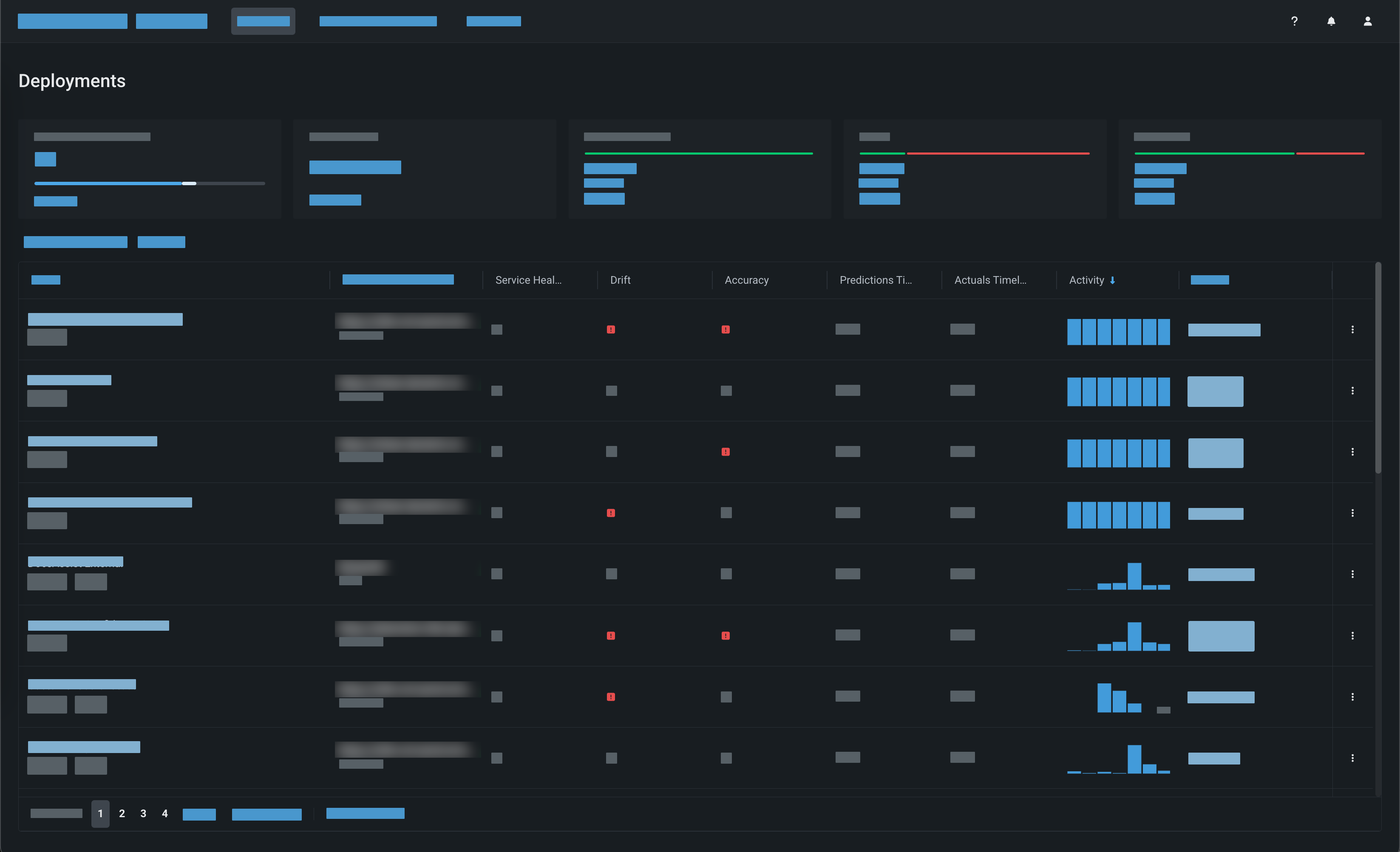
DataRobot uses a variety of metrics to monitor your deployment. Use the application's visualizations to track data (feature) drift, accuracy, bias, service health, and many more. You can set up notifications so that you are regularly informed of the model's status.
Tip
Consider enabling automatic retraining to automate an end-to-end workflow. With automatic retraining, DataRobot regularly tests challenger models against the current best model (the champion model) and replaces the champion if a challenger outperforms it.
Which visualizations should I use?
DataRobot provides many visualizations for analyzing models. Not all visualization tools are applicable to all modeling experiments—the visualizations you can access depend on your experiment type. The following table lists experiment types and examples of visualizations that are suited to their analysis:
| Experiment type | Analysis tools |
|---|---|
| All models |
|
| Regression |
|
| Classification |
|
| Time-aware modeling (time series and out-of-time validation) |
|
| Multiseries | Series Insights: Provides a histogram and table for series-specific information. |
| Segmented modeling | Segmentation tab: Displays data about each segment of a Combined Model. |
| Multilabel modeling | Metric values: Summarizes performance across labels for different values of the prediction threshold (which can be set from the page). |
| Image augmentation |
|
| Text AI |
|
| Geospatial AI |
|
| Clustering |
|
| Anomaly detection |
|