Ingest data with AWS Athena
Multiple big data formats now offer different approaches to compressing large amounts of data for storage and analytics; some of these formats include Orc, Parquet, and Avro. Using and querying these datasets can present some challenges. This section shows one way for DataRobot to ingest data in Apache Parquet format that is sitting at rest in AWS S3. Similar techniques can be applied in other cloud environments.
Parquet overview
Parquet is an open source columnar data storage format. It is often misunderstood to be used primarily for compression. Additionally, note that using compressed data introduces a CPU cost to both compress and decompress it; there's no speed advantage when using all of the data either. Snowflake addresses this in an article showing several approaches to load 10TB of benchmark data.
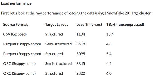
Snowflake demonstrates the load of full data records to be far higher for a simple CSV format. So what is the advantage of Parquet?
Columnar data storage offers little to no advantage when you are interested in a full record. The more columns requested, the more work must be done to read and uncompress them. This is why the full data exercise displayed above shows such a high performance for basic CSV files. However, selecting a subset of the data is where columnar really shines. If there are 50 columns of data in a loan dataset and the only one of interest is the loan_id, reading a CSV file will require reading 100% of the data file. However, reading a parquet file requires reading only 1 of 50 columns. Assume for simplicity's sake that all of the columns take up exactly the same space—this would translate into needing to read only 2% of the data.
You can make further read reductions by partitioning the data. To do so, create a path structure based on data values for a field. The SQL engine WHERE clause is applied to the folder path structure to decide whether a Parquet file inside it needs to be read. For example, you could partition and store daily files in a structure of YYYY/MM/DD for a loans datasource:
loans/2020/1/1/jan1file.parquet
loans/2020/1/2/jan2file.parquet
loans/2020/1/3/jan3file.parquet
The "hive style" of this would include the field name in the directory (partition):
loans/year=2020/month=1/day=1/jan1file.parquet
loans/year=2020/month=1/day=2/jan2file.parquet
loans/year=2020/month=1/day=3/jan3file.parquet
If the original program was only interested in the loan_id and specifically those loan_id values from January 2, 2020, then the 2% read would be reduced further still. Evenly distributed, this would reduce the read and decompress operation down to just 0.67% of the data, resulting in a faster read, a faster return of the data, and a lower bill for the resources required to retrieve the data.
Data for project creation
Find the data used in this page's examples on GitHub. The dataset uses 20,000 records of loan data from LendingClub and was uploaded to S3 using the AWS Command Line Interface.
aws --profile support s3 ls s3://engineering/athena --recursive | awk '{print $4}'
athena/
athena/ loan_credit /20k_loans_credit_data.csv
athena/ loan_history /year=2015/1/1020de8e664e4584836c3ec603c06786.parquet
athena/loan_history/year=2015/1/448262ad616e4c28b2fbd376284ae203.parquet
athena/loan_history/year=2015/2/5e956232d0d241558028fc893a90627b.parquet
athena/loan_history/year=2015/2/bd7153e175d7432eb5521608aca4fbbc.parquet
athena/loan_history/year=2016/1/d0220d318f8d4cfd9333526a8a1b6054.parquet
athena/loan_history/year=2016/1/de8da11ba02a4092a556ad93938c579b.parquet
athena/loan_history/year=2016/2/b961272f61544701b9780b2da84015d9.parquet
athena/loan_history/year=2016/2/ef93ffa9790c42978fa016ace8e4084d.parquet
20k_loans_credit_data.csv contains credit scores and histories for every loan. Loans are partitioned by year and month in impartial hive format to demonstrate the steps to work with either format within AWS Athena. Multiple parquet files are represented within the YYYY/MM structure, potentially representing different days a loan was created. All .parquet files represent loan application and repayment. This data is in a bucket in the AWS Region US-East-1 (N. Virginia).
AWS Athena
AWS Athena is a managed service on AWS that provides serverless access to use ANSI SQL against S3 objects. It uses Apache Presto and can read the following file formats:
- CSV
- TSV
- JSON
- ORC
- Apache Parquet
- Avro
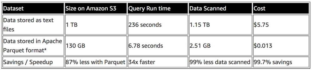
Athena also has support for compressed data in Snappy, Zlib, LZO, and GZIP formats. It charges on a pay-per-query model based on the amount of data read. AWS also provides an article on using Athena against both regular text files, as well as parquet, describing the amount of data read, time taken, and cost spent for a query:
AWS Glue
AWS Glue is an Extract Transform Load (ETL) tool that supports the workflow captured in this example. ETL jobs are not constructed and scheduled out. Use Glue to discover files and structure on the hosted S3 bucket in order to apply a high-level schema against the contents, so that Athena is able to understand how to read and query the contents. Glue stores contents in a hive-like meta store. Hive DDL can be written explicitly, but this example assumes a large number of potentially different files and leverages Glue's crawler to discover schemas and define tables.
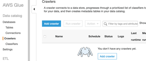
AWS Glue makes a crawler and points it at an S3 bucket. The crawler is set to output its data into an AWS Glue Data Catalog which is then leveraged by Athena. The Glue job should be created in the same region as the AWS S3 bucket (US-East-1 for the example on this page). This process is outlined below.
-
Click Add crawler in the AWS Glue service in the AWS console to add a crawler job.
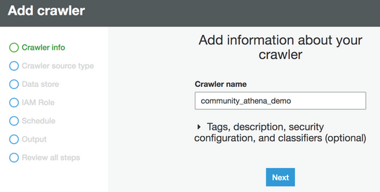
-
Name the crawler.
-
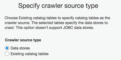
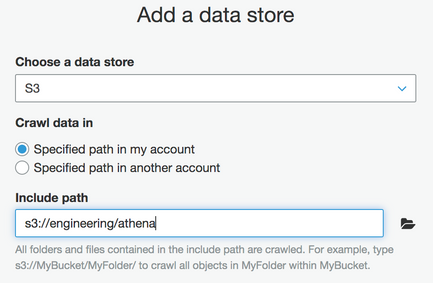
Choose the Data stores type and specify the bucket of interest.
-
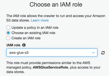
Choose or create an Identity and Access Management (IAM) role for the crawler. Note that managing IAM is out of scope for this example, but you can reference AWS documentation for more information about IAM privileges.
-
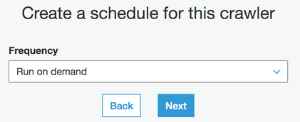
Set the frequency to run on demand, or update as necessary to meet requirements.
-
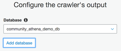
The crawler-discovered metadata needs to write to a destination. Choose a new or existing database to serve as a catalog.
Crawler creation can now be completed. A prompt asks if the demand crawler should be run now; choose Yes. In this example, you can see the crawler has discovered and created two tables for the paths:
loan_creditandloan_history.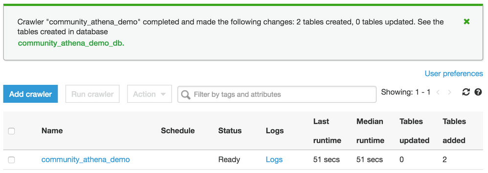
The log shows the created tables as well as partitions for the
loan_history.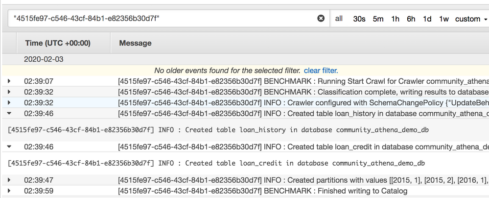
The year partition was left in Hive format while the month was not, to show what happens if this methodology is not applied. Glue assigns it a generic name.
-
Navigate to tables and open
loan_history.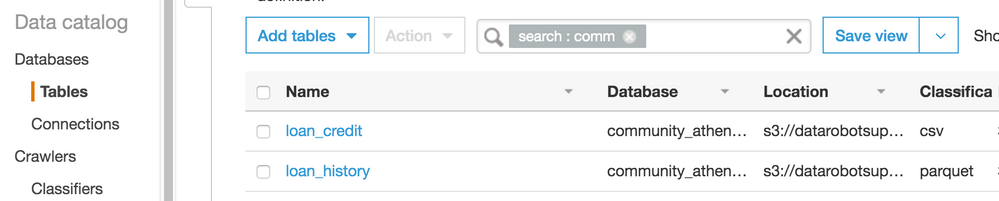
-
Choose to edit the schema and click on the column name to rename the secondary partition to month and save.
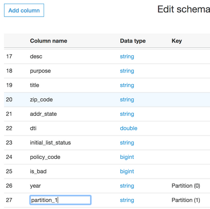
This table is now available for querying in Athena.
Create a project in DataRobot
This section outlines four methods for starting a project with data queried through Athena. All programmatic methods will use the Python SDK and some helper functions as defined in these DataRobot Community GitHub examples.
The four methods of providing data are:
- JDBC Driver
- Retrieve SQL results locally
- Retrieve S3 CSV results locally
- AWS S3 bucket with a signed URL
JDBC Driver
You can install JDBC drivers and use them with DataRobot to ingest data (contact Support for installation assistance for the driver, which is not addressed in this workflow). As of DataRobot 6.0 for the managed AI Platform offering, version 2.0 of the JDBC driver is available. Specifically, 2.0.5 is installed and available on the cloud. A catalog item dataset can be constructed by navigating to AI Catalog > Add New Data and then selecting Data Connection > Add a new data connection.
For the purposes of this example, the Athena JDBC driver connection is set up to explicitly specify the address. Awsregion and S3OutputLocation (required) are also specified. Once configured, query results write to this location as a CSV file.
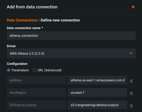
Authentication takes place with an AWSAccessKey and AWSSecretAccessKey for user and password on the last step. As AWS users often have access to many services, including the ability to spin up many resources, a best practice is to create an IAM account within AWS with specific permissions for querying and then only work with Athena and S3.
After creating the data connection, select it in the Add New Data from Data Connection modal and use it to create an item and project.
Retrieve SQL results locally
The snippet below sends a query to retrieve the first 100 records of loan history from the sample dataset. The results are provided back in a dictionary after paginating through the result set from Athena and loading it to local memory. You can then load the results to a dataframe, manipulate it to engineer new features, and push it into DataRobot to create a new project. The s3_out variable is a required parameter for Athena, which is where Athena writes CSV query results. This file is used in subsequent examples.
athena_client = session.client('athena')
database = 'community_athena_demo_db'
s3_out = 's3://engineering/athena/output/'
query = "select * from loan_history limit 100"

query_results = fetchall_athena_sql(query, athena_client, database, s3_out)

# Convert to dataframe to view and manipulate
df = pd.DataFrame(query_results)
df.head(2)

proj = dr.Project.create(sourcedata=df,
    project_name='athena load query')

# Continue work with this project via the DataRobot python package, or work in GUI using the link to the project printed below
print(DR_APP_ENDPOINT[:-7] + 'projects/{}'.format(proj.id))
DataRobot only recommends this method for smaller-sized datasets; it may be both easier and faster to simply download the data as a file rather than spool it back in paginated query results. The method uses a pandas DataFrame for convenience and ease of potential data manipulation and feature engineering; it is not required for working with the data or creating a DataRobot project. Additionally, note that the machine that this code runs on requires adequate memory to work with a pandas DataFrame for the size of the dataset being used in this example.
Retrieve S3 CSV results locally
The snippet below shows a more complicated query than the method above. It pulls all loans and joins CSV credit history data with Parquet loan history data. Upon completion, the S3 results file itself is downloaded to a local Python environment. From here, additional processing can be performed or the file can be pushed directly to DataRobot for a new project as shown in the snippet.
athena_client = session.client('athena')
s3_client = session.client('s3')
database = 'community_athena_demo_db'
s3_out_bucket = 'engineering'
s3_out_path = 'athena/output/'
s3_out = 's3://' + s3_out_bucket + '/' + s3_out_path
local_path = '/Users/mike/Documents/community/'
local_path = !pwd
local_path = local_path[0]

query = "select lh.loan_id, " \
    "lh.loan_amnt, lh.term, lh.int_rate, lh.installment, lh.grade, lh.sub_grade, " \
    "lh.emp_title, lh.emp_length, lh.home_ownership, lh.annual_inc, lh.verification_status, " \
    "lh.pymnt_plan, lh.purpose, lh.title, lh.zip_code, lh.addr_state, lh.dti, " \
    "lh.installment / (lh.annual_inc / 12) as mnthly_paymt_to_income_ratio, " \
    "lh.is_bad, " \
    "lc.delinq_2yrs, lc.earliest_cr_line, lc.inq_last_6mths, lc.mths_since_last_delinq, lc.mths_since_last_record, " \
    "lc.open_acc, lc.pub_rec, lc.revol_bal, lc.revol_util, lc.total_acc, lc.mths_since_last_major_derog " \
    "from community_athena_demo_db.loan_credit lc " \
    "join community_athena_demo_db.loan_history lh on lc.loan_id = lh.loan_id"

s3_file = fetch_athena_file(query, athena_client, database, s3_out, s3_client, local_path)

# get results file from S3
s3_client.download_file(s3_out_bucket, s3_out_path + s3_file, local_path + '/' + s3_file)

proj = dr.Project.create(local_path + '/' + s3_file,
    project_name='athena load file')

# further work with project via the python API, or work in GUI (link to project printed below)
print(DR_APP_ENDPOINT[:-7] + 'projects/{}'.format(proj.id))
AWS S3 bucket with a signed URL
Another method for creating a project in DataRobot is to ingest data from S3 using URL ingest. There are several ways this can be done based on the data, environment, and configuration used. This example leverages a private dataset on the cloud and creates a Signed URL for use in DataRobot.
| Dataset | DataRobot Environment | Approach | Description |
|---|---|---|---|
| Public | Local install, Cloud | Public | If a dataset is in a public bucket, the direct HTTP link to the file object can be ingested. |
| Private | Local install | Global IAM role | You can install DataRobot with an IAM role granted to the DataRobot service account that has its own access privileges to S3. Any URL passed in that the DataRobot service account can see can be used to ingest data. |
| Private | Local install | IAM impersonation | You can implement finer-grained security control by having DataRobot assume the role and S3 privileges of a user. This requires LDAP authentication and LDAP fields containing S3 information be made available. |
| Private | Local install, Cloud | Signed S3 URL | AWS users can create a signed URL to an S3 object, providing a temporary link that expires after a specified amount of time. |
The snippet below builds on the work presented in the method to retrieve S3 CSV results locally. Rather than download the file to a local environment, you can use AWS credentials to sign the URL for temporary usage. The response variable contains a link to the results file, with an authentication string good for 3600 seconds. Anyone with the entire string URL will be able to access the file for the duration requested. In this way, rather than downloading the results locally, a DataRobot project can be initiated by referencing the URL value.
response = s3_client.generate_presigned_url('get_object',
    Params={'Bucket': s3_out_bucket,
            'Key': s3_out_path + s3_file},
    ExpiresIn=3600)

proj = dr.Project.create(response,
    project_name='athena signed url')

# further work with project via the python API, or work in GUI (link to project printed below)
print(DR_APP_ENDPOINT[:-7] + 'projects/{}'.format(proj.id))
Helper functions and full code is available in the DataRobot Community GitHub repo.
Wrap-up
After using any of the methods detailed above, your data should be ingested in DataRobot. AWS Athena and Apache Presto have enabled SQL against varied data sources to produce results that can be used for data ingestion. Similar approaches can be used to work with this type of input data in Azure and Google cloud services as well.