Price elasticity of demand modeling
The price elasticity of demand is a measurement for how demand for a product is affected by changes in its price, and is a crucial consideration for organizations that make pricing decisions. Generally, there’s an inverse relationship between price and demand; as price for a product or category increases, demand or the number of products sold tends to decrease. However, not all products are equally sensitive to changes in price. Factors such as product differentiation, competition, and promotional activities all play pivotal roles in the relationship between price and demand for individual products or categories. To maximize profits, companies must use price elasticities to determine the optimal balance between price and demand, as well as monitor these elasticities regularly to account for changes in the overall market environment.
The included notebook helps you to understand the impact that changes in price will have on consumer demand for a given product. Business analysts that measure price elasticity and business users that require elasticity as an input to make pricing decisions will benefit from this notebook.
Following this workflow will allow you to identify relationships between price and demand, maximize revenue by properly pricing products, monitor price elasticities for changes in price and demand, and reduce manual processes used to obtain and update price elasticities.
Solution value
Traditional approaches to calculating price elasticity leave much to be desired:
- They are often managed by third-party analytics providers, obscuring methods and limiting experimentation.
- Category expertise is missing in selecting confounding variables.
- Single coefficients do not fully capture a price’s relationship to demand and require better model explainability.
- Models are typically limited to linear methods, limiting their quality and accuracy.
- The traditional approach is a single point-in-time estimate, but with high-quality model monitoring and retraining this can be a living and dynamic analysis.
Using DataRobot for price elasticity modeling provides a much more flexible and accurate way to make pricing decisions.
The primary issues that this use case addresses include:
- Revenue loss due to non-optimally priced items.
- Increased cadence for analyzing pricing with greater user control and understanding.
- Decreased reliance on expensive third-party analytics vendors.
Data overview
Each row in this use case's dataset represents a product, by day, in a single market, with sales and a price information. The same product on the same day in a different market is represented in an independent row. Additionally, confounding variables related to active promotions, weather, and macroeconomic indicators are added to help isolate the relationship between price and sales. These should be reduced or augmented based on your category or product knowledge.
Feature overview
- Date: calendar date, daily level
- SKUName: unique identifier for each product
- Sales: Total dollar sales for that product for that date
- PriceBaseline: Price of product without discounting
- PriceActual: Current price of product with discounting
- PctOnSale: Percentage difference between PriceBaseline and PriceActual
- HotDay: Binary for whether the temperature was above some threshold
- sunnDay: Binary for if the day was sunny for a given geography
- EconChangeGDP: Percentage change in US GDP reported quarterly (blank on unreported dates)
- EconJobsChange: Percentage change in US unemployment insurance claims, available weekly (blank on unreported dates)
- AnnualizedCPI: Federal Reserve measure of national price inflations, available monthly
Prepare data
Use DataRobot’s EDA stages to proactively identify common impediments to model performance like outliers, missing values, and target leakage.
Build feature lists to approach modeling with the appropriate variables. For this project, DataRobot uses the provided dates and creates variables for the Day of the Week, Day of the Month, the Month, and the Year.
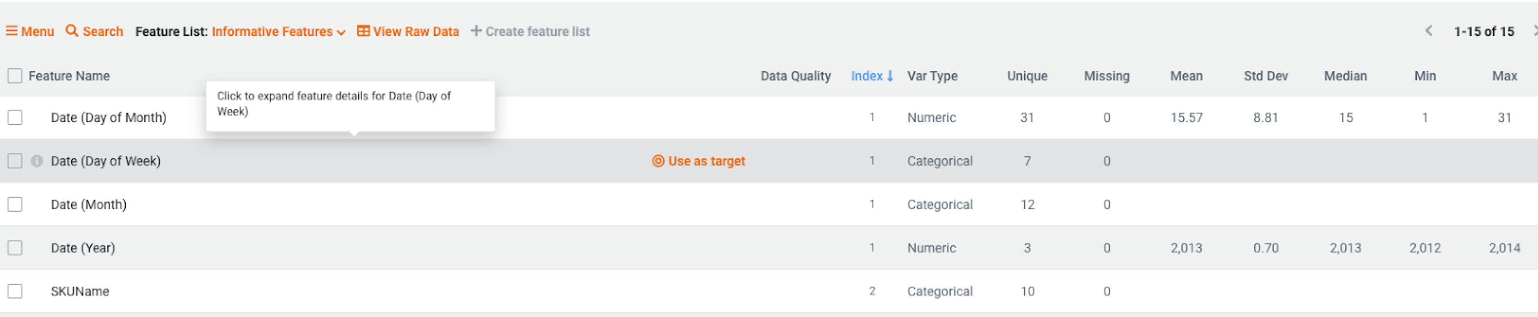
This use case removes Year and keeps all other variables. This use case also creates a feature list of variables that should always have a negative relationship with sales (monotonically decreasing and uses its relationship to inform model training. In this case, the feature list enforces the idea that sales should always decrease as price increases.

Model insights
When modeling completes, identify the top performing model in the Leaderboard and use the Understand tab in the UI to learn more about the model’s behavior.
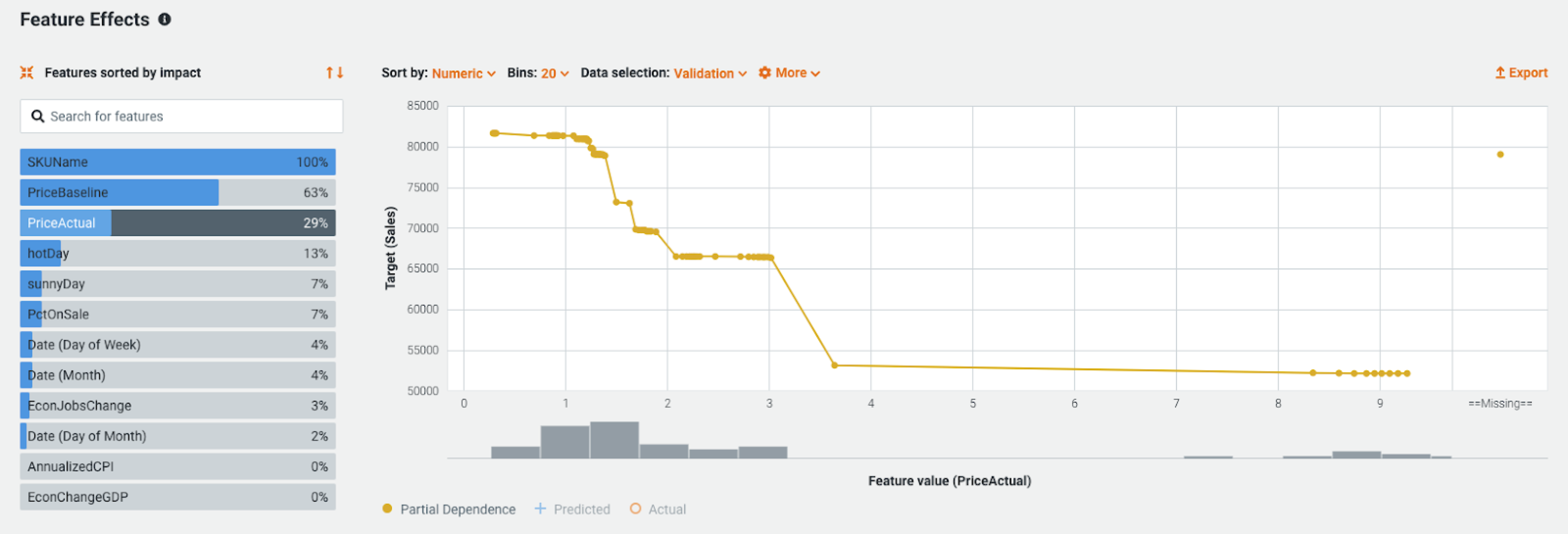
In the example below, the Feature Impact chart shows that the product, its price, and the associated marketing efforts have the highest feature importance. Also, two of the included macroeconomic indicators have little to no impact on the model. This is a case where experimentation by removing these two variables may improve model performance.

For this use case, the partial dependence plot shown in Feature Effects may be the most important model insight. In this case, the plot shows impact of price increases on sales at all price values. Rather than considering a single coefficient, this acknowledges that not all units of price increase have the same impact on sales. For example, in this graph a price increase from $2.10 to $3 has almost no effect on sales, but increasing the price beyond $3 has a significant negative impact.
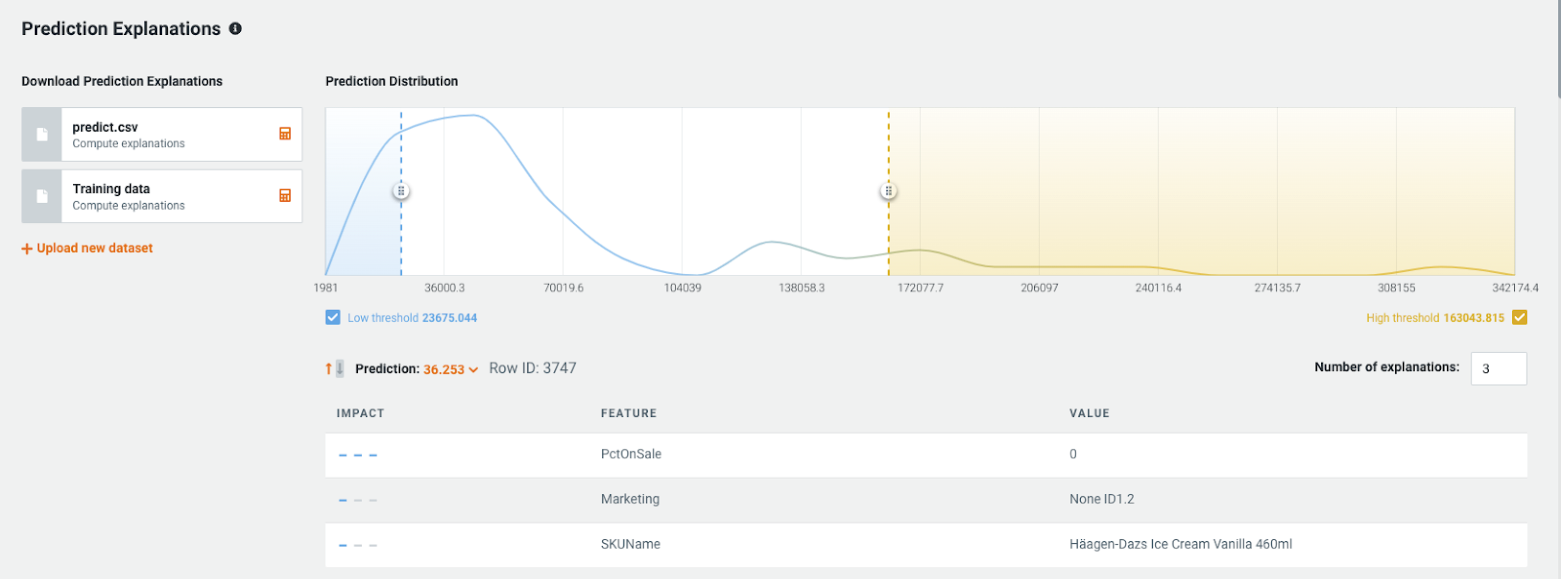
Prediction Explanations (XEMP in this example) are extremely useful to analysts to aid in answering “Why?” questions around their product or category. In the below example we can see a product with low expected sales. The top three reasons given show that this is because the item is not on sale and has no marketing activity to promote it. This is an ice cream, so there is likely a discounted brand with the same flavor close by, altering consumer decision making.
Optimizing price
With an understanding of how prices and other factors impact sales, you can find an optimal price that maximizes revenue. To do so, you can simulate many possible pricing scenarios for the products you want to analyze. The starting data contains one row for each product on an upcoming date, providing as much confounding information possible. The price to start is the currently planned price.
This example creates an observation of every product with 1% increments ranging from a 25% discount to a 25% price increase.

Use the top model from the Leaderboard to make predictions against the dataset and calculate the total revenue for each simulation.
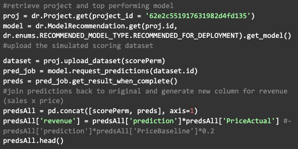
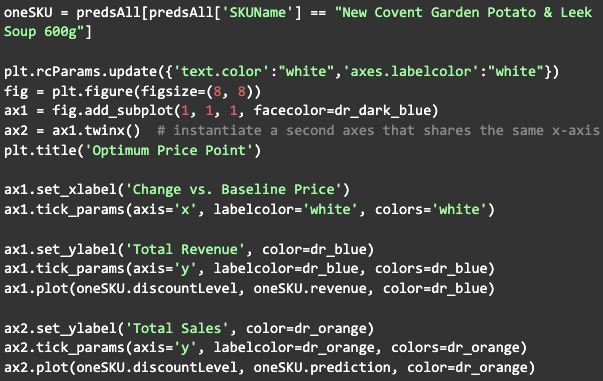
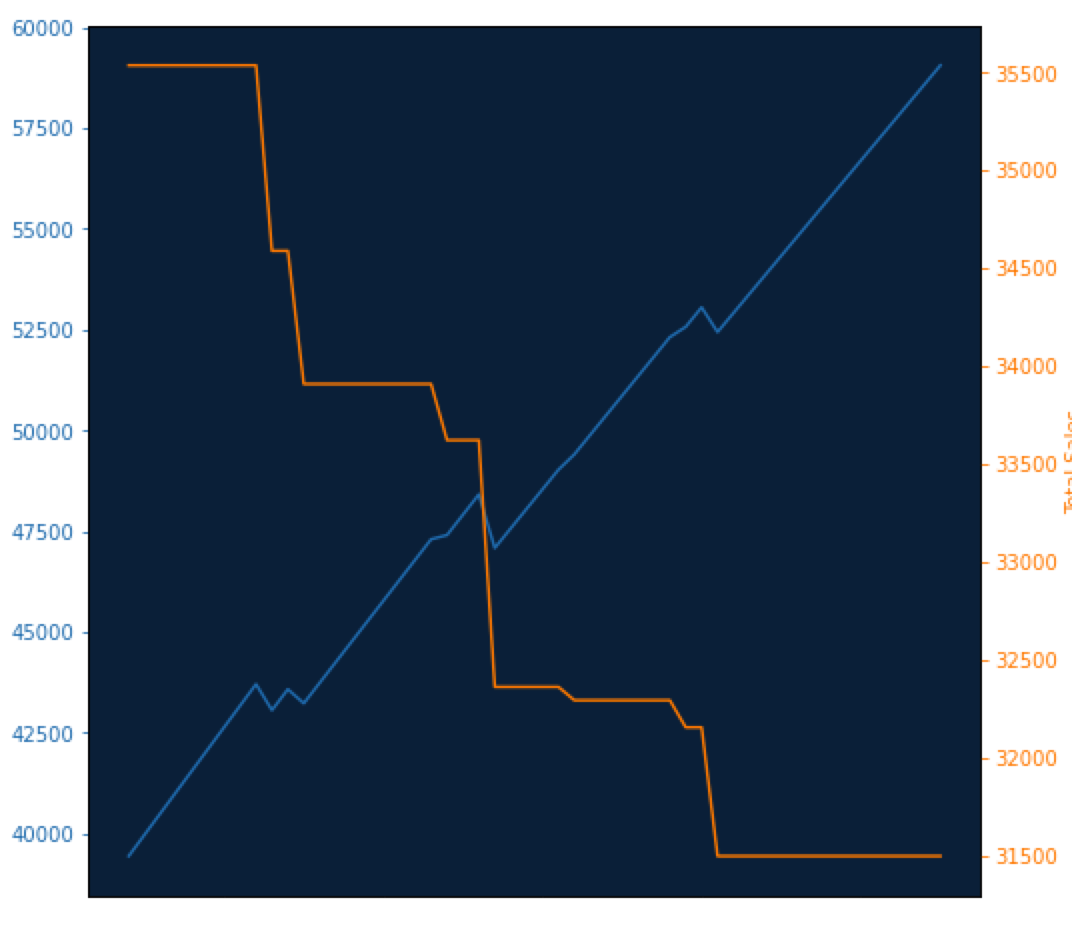
Select a single product and observe its unique relationship between price and sales. In this graph, note the intersection point between sales and revenue.
Lastly, calculate the optimum price point for each product that maximizes its revenue.
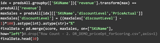
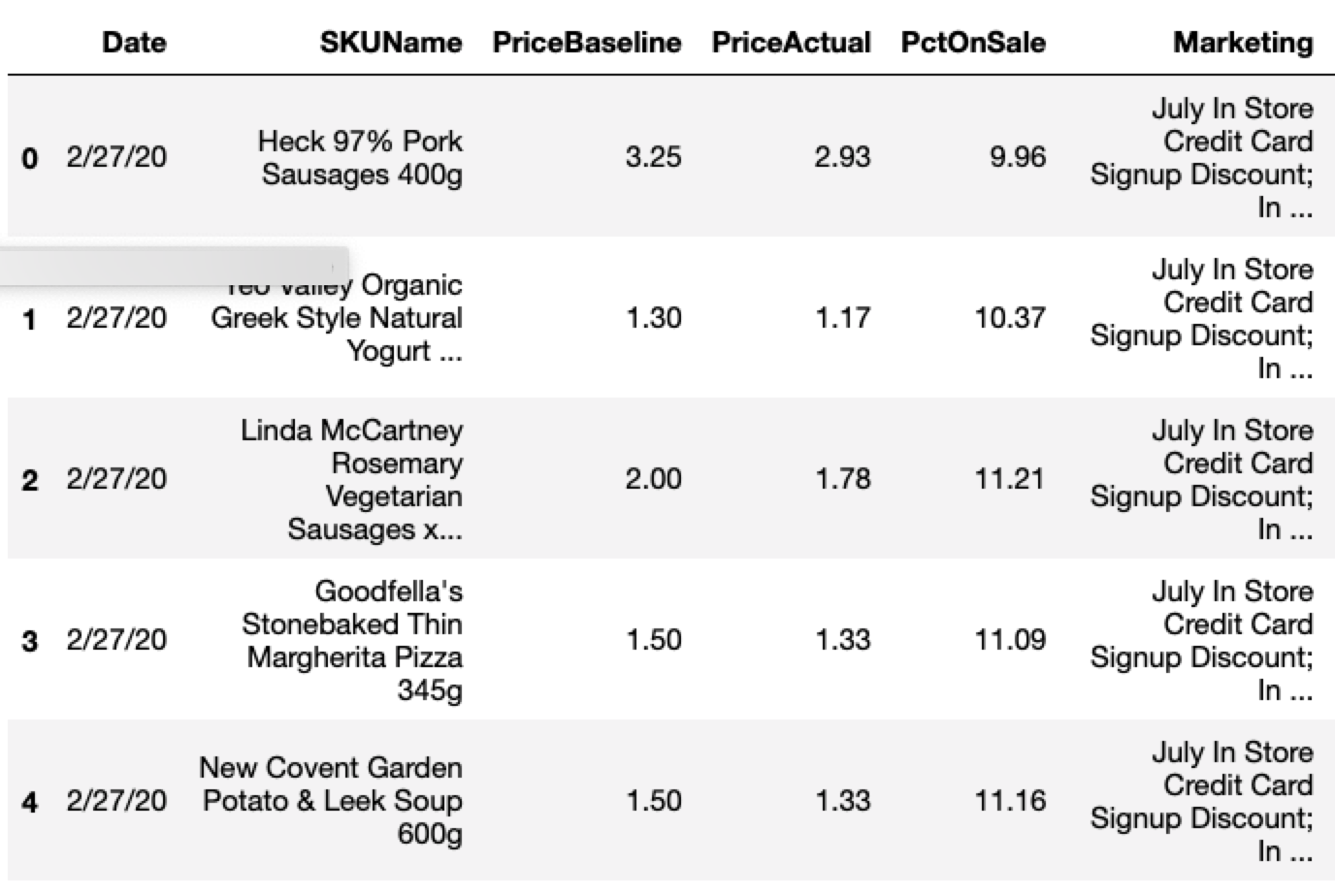
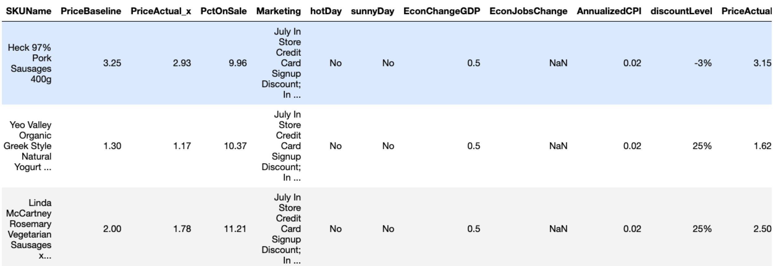
The final output shows a new optimal price point for each product under the column PriceActual_y. Note that Heck 97% Pork Sausages are actually being discounted too much:
Single elasticity coefficient
To generate a single coefficient for the PriceActual variable, use a different model from the model Leaderboard. Find the initial Linear Regression blueprint and retrain it on 100% of the data using the Holdout partition.

Once the Linear Regression model finishes retraining, select it and navigate to Describe > Coefficients to export its coefficients. Use the export button to download all coefficients and find the value associated with Price Actual.


Demo
See the notebook outlining this use case here.