Predict the likelihood of a loan default
This page outlines the use case to reduce defaults and minimize risk by predicting the likelihood that a borrower will not repay their loan. This use case is captured in:
- A Jupyter notebook that you can download and execute.
- A UI-based business accelerator.
Business problem
After the 2008 financial crisis, the IASB (International Accounting Standard Board) and FASB (Financial Accounting Standards Board) reviewed accounting standards. As a result, they updated policies to require estimated Expected Credit Loss (ECL) to maintain enough regulatory capital to handle any Unexpected Loss (UL). Now, every risk model undergoes tough scrutiny, and it is important to be aware of the regulatory guidelines while trying to deliver an AI model. This use case focuses on credit risk, which is defined as the likelihood that a borrower would not repay their lender. Credit risk can arise for individuals, SMEs, and large corporations and each is responsible for calculating ECL. Depending on the asset class, different companies take different strategies and components for calculation differ, but involve:
- Probability of Default (PD)
- Loss Given Default (LGD)
- Exposure at Default (EAD)
The most common approach for calculating the ECL is the following (see more about these factors in problem framing):
`ECL = PD * LGD * EAD`
This use case builds a PD model for a consumer loan portfolio and provides some suggestions related LGD and EAD modeling. Sample training datasets for using some of the techniques described here are publicly available on Kaggle, but for interpretability, the examples do not exactly represent the Kaggle datasets. Click here to jump directly to the hands-on sections that begin with working with data. Otherwise, the following several paragraphs describe the business justification and problem framing for this use case.
Solution value
Many credit decisioning systems are driven by scorecards, which are very simplistic rule-based systems. These are built by end-user organizations through industry knowledge or through simple statistical systems. Some organizations go a step further and obtain scorecards from third parties, which may not be customized for an individual organization’s book. An AI-based approach can help financial institutions learn signals from their own book and assess risk at a more granular level. Once the risk is calculated, a strategy may be implemented to use this information for interventions. If you can predict someone is going to default, this may lead to intervention steps, such as sending earlier notices or rejecting loan applications.
Problem framing
Banks deal with different types of risks, like credit risk, market risk, and operational risk. Calculating the ECL using ECL = PD * LGD * EAD is the most common approach. Risk is defined in financial terms as the chance that an outcome or investment’s actual gains will differ from an expected outcome or return.
There are many ways you can position the problem, but in this specific use case you will be building Probability of Default (PD) models and will provide some guidance related to LGD and EAD modeling. For the PD model, the target variable is is_bad. In the training data, 0 indicates the borrower did pay and 1 indicates they defaulted.
Here is additional guidance on the definition of each component of the ECL equation.
Probability of Default (PD)
- The borrower’s inability to repay their debt in full or on time.
- Target is normally defined as 90 days delinquency.
- Machine learning models generally give good results if adequate data is available for a particular asset class.
Loss Given Default (LGD)
- The proportion of the total exposure that cannot be recovered by the lender once a default has occurred.
- Target is normally defined as the recovery rates and the value lies between 0 and 1.
- Machine learning models required for this problem normally use Beta regression, which is not very common and therefore not supported in a lot of statistical software. We can divide this into two stages since a lot of the values in the target are zero.
- Stage 1—the model predicts the likelihood of recovery greater than zero.
- Stage 2—the model predicts the rate for all loans with the likelihood of recovery greater than zero.
Exposure at Default (EAD)
- The total value that a lender is exposed to when a borrower defaults.
- Target is the proportion from the original amount of the loan that is still outstanding at the moment when the borrower defaulted.
- Generally, machine learning models with MSE as loss are used.
ROI estimation
The ROI for implementing this solution can be estimated by considering the following factors:
- ROI varies on the size of the business and the portfolio. For example, the ROI for secured loans would be quite different to those for a credit card portfolio.
- If you are moving from one compliance framework to another, you need to take the appropriate considerations—whether to model a new and existing portfolio separately and, if so, make appropriate adjustments to the ROI calculations.
- ROI depends on the decisioning system. If it is a binary (yes or no) decision on loan approval, you can assign dollar values to the amounts of true positives, false positives, true negatives, and false negatives. The sum total of that is the value at a given threshold. If there is an existing model, the difference in results between existing and new models is the ROI captured.
- If the decisioning is non binary, then at every decision point, evaluate the difference between loan provided and the collections done.
Working with data
For illustrative purposes, this use case simplifies the sample datasets provided by Home Credit Group, which are publicly available on Kaggle.
Sample feature list
| Feature Name | Data Type | Description | Data Source | Example |
|---|---|---|---|---|
| Amount_Credit | Numeric | Credit taken by a person | Application | 20,000 |
| Flag_Own_Car | Categorical | Flag if applicant owns a car | Application | 1 |
| Age | Numeric | Age of the applicant | Application | 25 |
| CreditOverdue | Binomial | Whether credit is overdue | Bureau | TRUE |
| Channel | Categorical | Channel through which credit taken | PreviousApplication | Online |
| Balance | Numeric | Balance in credit card | CreditCard | 2,500 |
| Is_Bad | Numeric (target) | Whether the borrower defaulted, 0 or 1 | Bureau | 1 (default) |
Modeling and insights
DataRobot automates many parts of the modeling pipeline, including processing and partitioning the dataset, as described here. This use case skips the modeling section and moves straight to model interpretation. DataRobot provides a variety of insights to interpret results and evaluate-accuracy.
Interpret results
After automated modeling completes, the Leaderboard ranks each model. By default, DataRobot uses LogLoss as the evaluation metric.
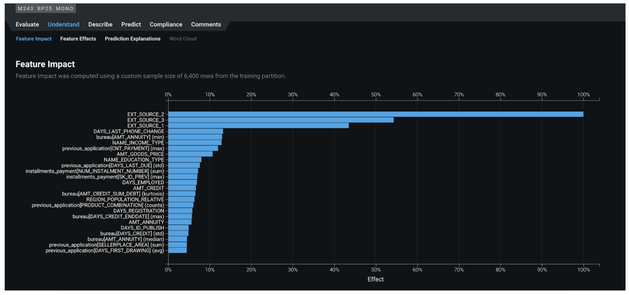
Feature Impact
Feature Impact reveals the association between each feature and the model target. For example:
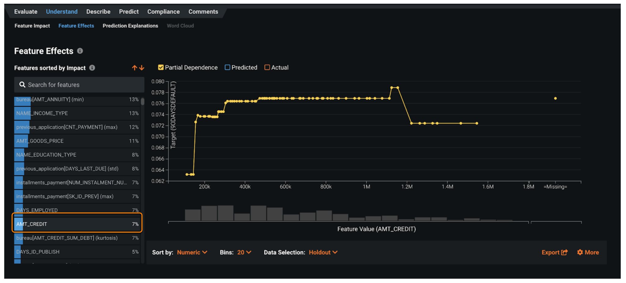
Feature Effects
To understand the direction of impact and the default risk at different levels of the input feature, DataRobot provides partial dependence plots as part of the Feature Effects visualization. It depicts how the likelihood of default changes when the input feature takes different values.
In this example, which is plotting for AMT_CREDIT (loan amount), as the loan amount increases above to $300K, the default risk increases in a step manner from 6% to 7% and then in another step to 7.8% when the loan about is around $500K.
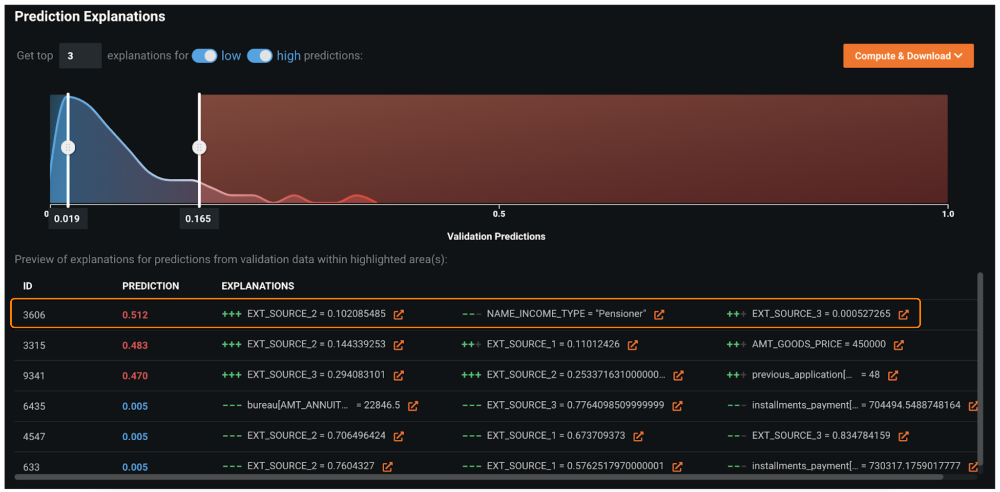
Prediction Explanations
In the Prediction Explanations visualization, DataRobot provides, for each alert scored and prioritized by the model, a human-interpretable rationale. In the example below, the record with ID=3606 gets a very high likelihood of turning into a loan default (prediction=51.2%). The main reasons are due to information from external sources (EXT_SOURCE_2 and EXT_SOURCE_3) and the source of income (NAME_INCOME_TYPE) being pension.
Prediction Explanations also help in maintaining regulatory compliance. It provides reasons why a particular loan decision was taken.
Evaluate accuracy
The following insights help evaluate accuracy.
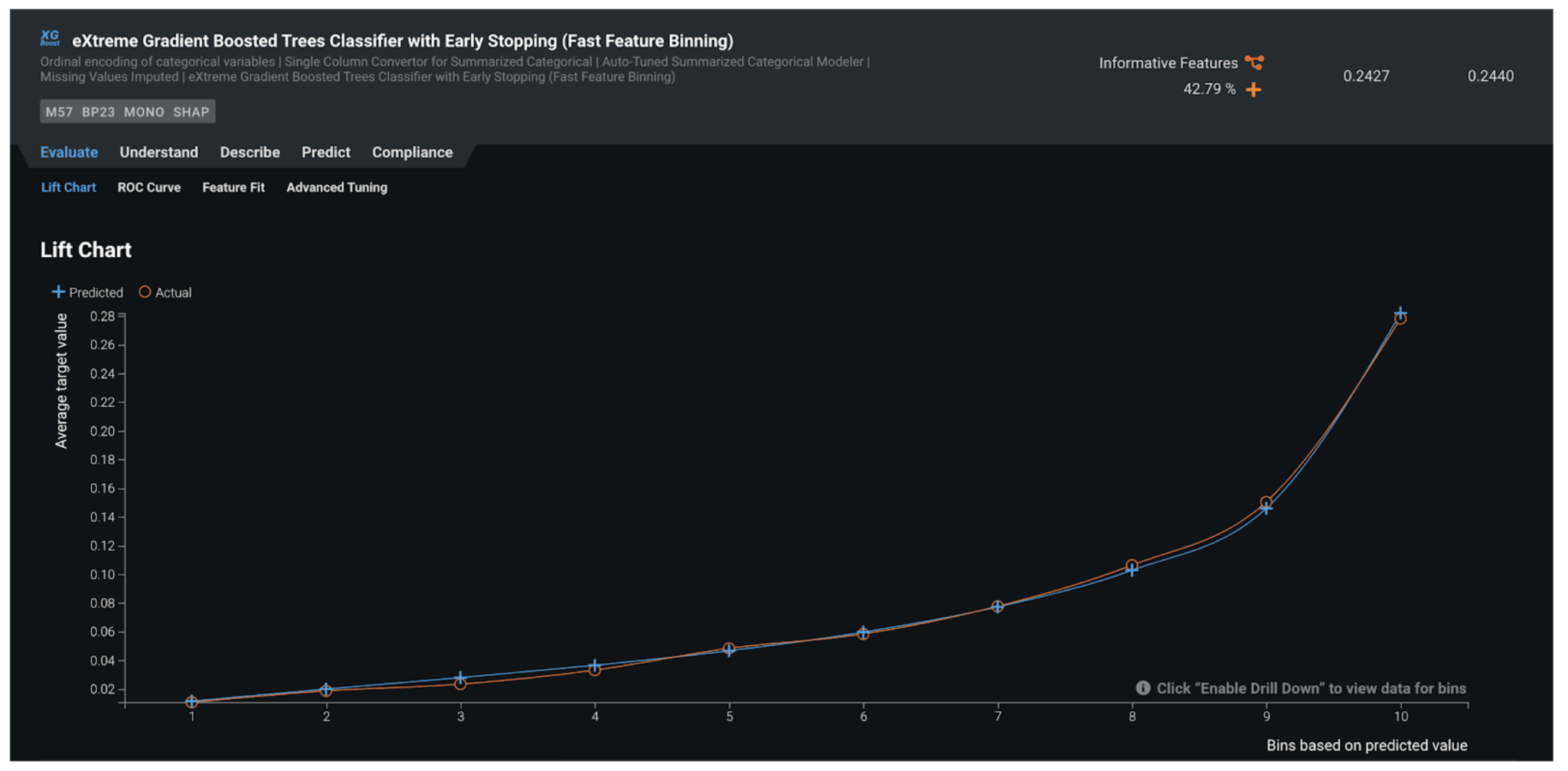
Lift Chart
The Lift Chart shows you how effective the model is at separating the default and non-default applications. Each record in the out-of-sample partition gets scored by the trained model and assigned with a default probability. In the Lift Chart, records are sorted based on the predicted probability, broken down into 10 deciles, and displayed from lowest to the highest. For each decile, DataRobot computes the average predicted risk (blue line/plus) as well as the average actual risk (orange line/circle), and displays the two lines together. In general, the steeper the actual line is, and the more closely the predicted line matches the actual line, the better the model is. A consistently increasing line is another good indicator.
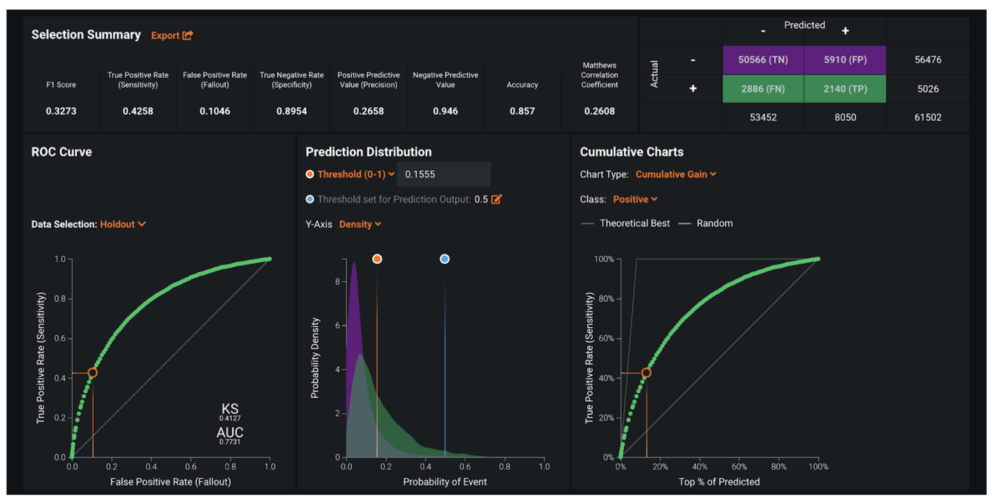
ROC Curve
Once you know the model is performing well, select an explicit threshold to make a binary decision based on the continuous default risk predicted by DataRobot. The ROC Curve tools provide a variety of information to help make some of the important decisions in selecting the optimal threshold:
- The false negative rate has to be as small as possible. False negatives are the applications that are flagged as not defaults but actually end up defaulting on payment. Missing a true default is dangerous and expensive.
- Ensure the selected threshold is working not only on the seen data, but on the unseen data too.
Post-processing
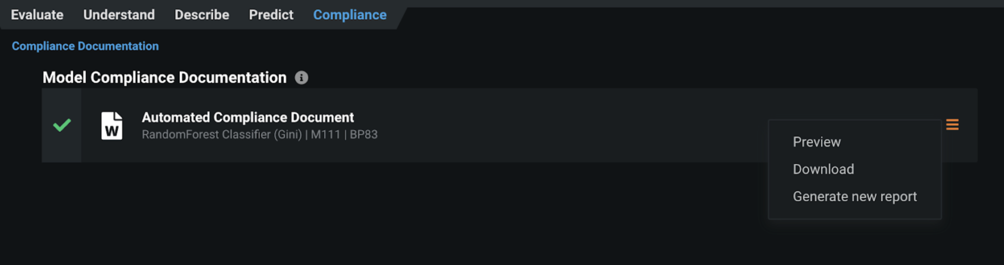
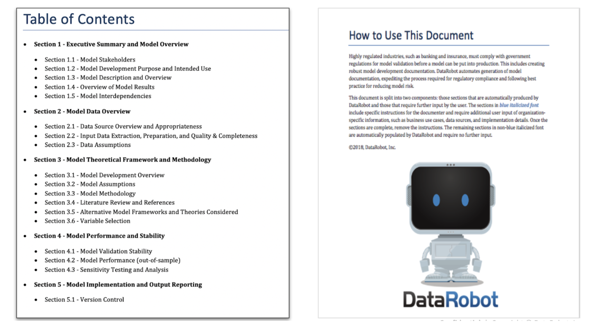
In some cases where there are fewer regulatory considerations, straight-through processing (SIP) may be possible, where an automated yes or no decision can be taken based on the predictions. But the more common approach is to convert the risk probability into a score (i.e., a credit score determined by organizations like Experian and TransUnion). The scores are derived based on exposure of probability buckets and on SME knowledge. Most of the machine learning models used for credit risk require approval from the Model Risk Management (MRM) team; to address this, the Compliance Report provides comprehensive evidence and rationale for each step in the model development process.
Predict and deploy
After finding the right model that best learns patterns in your data, you can deploy the model into your desired decision environment. Decision environments are the ways in which the predictions generated by the model will be consumed by the appropriate stakeholders in your organization, and how these stakeholders will make decisions using the predictions to impact the overall process. Decisions can be a blend of automated and straight-through processing or manual interventions. The degree of automation depends on the portfolio and business maturity. For example, retail loans or peer-to-peer portfolios in banks and fintechs are highly automated. Some fintechs promote their low loan-processing times. Unlike high ticket items, like mortgages, corporate loans may be a case of manual intervention.
Decision stakeholders
The following table lists potential decision stakeholders:
| Stakeholder | Description |
|---|---|
| Decision Executors | The underwriting team will be the direct consumers of the predictions. These can be direct systems in the case of straight-through processing or an underwriting team sitting in front offices in the case of manual intervention. |
| Decision Managers | Decisions often flow through to the Chief Risk Officer, who is responsible for the ultimate risk of the portfolio. However, there generally are intermediate managers (based on the structure of the organization). |
| Decision Authors | Data scientists in credit risk teams drive the modeling. The model risk monitoring team is also be a key stakeholder. |
Decision process
Generally, models do not result in a direct yes or no decision being made, except in cases where models are used in less-regulated environments. Instead, the risk is converted to a score and, based on the score, impacts the interest or credit amount offered to the customer.
Model monitoring
Predictions are done in real time or batch mode based on the nature of the business. Regular monitoring and alerting is critical for data drift. This is particularly important from a model risk perspective. These models are designed to be robust and last longer, so recalibration may be less frequent than in other industries.
Implementation considerations
- Credit risk models normally require integrations with third-party solutions like Experian and FICO. Ask about deployment requirements and if it is possible to move away from legacy tools.
- Credit risk models require approval from the validation team, which can take significant time (for example, convincing them to adopt new model approval methods if they have not previously approved machine learning models).
- Model validation teams can have strict requirements for specific assets. For example, if models need to generate an equation and therefore model code export. Be certain to discuss any questions in advance with the modeling team before taking the final model to validation teams.
- Discuss alternative approaches for assets where the default rate was historically low, as the model might not be accurate enough to prove ROI.
In addition to traditional risk analysis, target leakage may require attention in this use case. Target leakage can happen when information that should not be available at the time of prediction is being used to train the model. That is, particular features leak information about the eventual outcome, and that artificially inflates the performance of the model in training. While the implementation outlined in this document involves relatively few features, it is important to be mindful of target leakage whenever merging multiple datasets due to improper joins. DataRobot supports robust target leakage detection in the second round of exploratory data analysis (EDA) and the selection of the Informative Features feature list during Autopilot.
Demo
See the notebook here or the UI-based accelerator here.