Error metrics
Eureqa error metrics are measures of how well a Eureqa model fits your data. When DataRobot performs Eureqa model tuning, it searches for models that optimized error and complexity. The error metric that best defines a well-fit model will depend on the nature of the data and the objectives of the modeling exercise. DataRobot supports a variety of different error metrics for Eureqa models.
Error metric selection and configuration determines how DataRobot will assess the quality of potential solutions. DataRobot sets default error metrics for each model, but advanced users can choose to optimize for different error metrics. Changing error metrics settings changes how DataRobot optimizes its solutions.
The Error Metric parameter, error_metric, is available within the Prediction Model Parameters and can be modified as part of tuning your Eureqa models. Available error metrics are listed for selection.

DataRobot versus Eureqa
Note
There is some overlap in the DataRobot optimization metrics and Eureqa error metrics. You may notice, however, that in some cases the metric formulas are expressed differently. For example, predictions may be expressed as y^ versus f(x). Both are correct, with the nuance being that y^ often indicates a prediction generally, regardless of how you got there, while f(x) indicates a function that may represent an underlying equation.
DataRobot provides the optimization metrics for setting error metrics at the project level. The optimization metric is used to evaluate the error values shown on the Leaderboard entry for all models (including Eureqa), to compare different models, and to sort the Leaderboard.
By contrast, the Eureqa error metric specifically governs how the Eureqa algorithm is optimized for the related solution and is not a project-level setting. When configuring these metrics, keep in mind they are fully independent and, in general, setting either metric does not influence the other metric.
Choose a Eureqa error metric
The best error metric for your problem will depend on your data and the objectives of your modeling analysis. For many problems there isn't one correct answer; therefore, DataRobot recommends running models with several different error metrics to see what types of models will be produced and which results best align with the modeling objectives.
When choosing an error metric, consider these suggestions for setting and configuring error metrics.
Error metric parameters
Mean Absolute
The mean of the absolute value of the residuals. A smaller value indicates a lower error.
Details: Mean Absolute Error is calculated as:
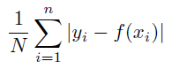
How it's used: To minimize the residual errors. Mean Absolute Error is a good general purpose error metric, similar to Mean Squared Error but more tolerant of outliers. It is a common measure of forecast error in time series analyses. The value of this metric can be interpreted as the average distance predictions are from the actual values.
Considerations:
- Assumes the noise follows a double exponential distribution.
- Compared to Mean Squared Error, Mean Absolute Error tends to be more permissive of outliers and can be a good choice if outliers are being given too much weight when optimizing for MSE.
- Can be interpreted as the average error between predictions and actuals of the model.
Mean Absolute Percentage
The mean of the absolute percentage error. A smaller value indicates a lower error. Note that rows for which the actual value of the target variable = 0 are excluded from the error calculation.
Details: Mean Absolute Percentage Error is calculated as:
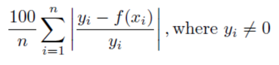
How it's used: To minimize the absolute percentage error. MAPE is a common measure of forecast error in time series forecasting analyses. The value of this metric can be interpreted as the average percentage that predictions vary from the actual values.
Considerations:
- Mean Absolute Percentage Error will be undefined when the actual value is zero. Eureqa’s calculation excludes rows for which the actual value is zero.
- Mean Absolute Percentage Error is extremely sensitive to very small actual values - high percentage errors on small values may dominate the error metric calculation.
- Can be interpreted as the average percentage that predicted values vary from actual values.
- Mean Absolute Percentage Error may bias a model to underestimate actual values.
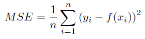
Mean Squared
The mean of the squared value of the residuals. A smaller value indicates a lower error.
Details: Mean Squared Error is calculated as:
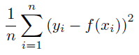
How it's used: to minimize the squared residual errors. Mean Squared Error is the most common error metric. It emphasizes the extreme errors, so it's more useful if you have concerns about large errors with greater consequences.
Considerations:
- It assumes that the noise follows a normal distribution.
- It's tolerant of small deviations, and sensitive to outliers.
- For classification problems, logistic models optimized for Mean Squared Error produce values which can be interpreted as predicted probabilities.
- Optimizing for Mean Squared Error is equivalent to optimizing for R^2.
Root Mean Squared
The mean of the squared value of the residuals. A smaller value indicates a lower error.
Details: Root Mean Squared Error is calculated as:
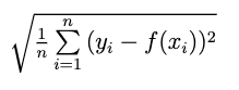
How it's used: to minimize the squared residual errors. Root Mean Squared Error is used similarly to Mean Squared Error. Root Mean Squared Error de-emphasizes extreme errors as compared to Mean Squared Error, so it is less likely to be swayed by outliers but more likely to favor models that have many records that do a little better and a few that do a lot worse.
Considerations:
- It assumes that the noise follows a normal distribution.
R^2 Goodness of Fit (R^2)
The percentage of variance in the target variable that can be explained by the model. A higher value indicates a better fit.
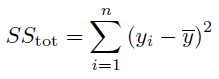
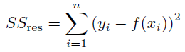
Details: R^2 is calculated as:
to give the fraction of variance explained. This value is multiplied by 100 to give the percentage of variance explained.
SStot is proportional to the total variance, and SSres is the residual sum of squares (proportional to the unexplained variance).
How it's used: to maximize the explained variance. It is the equivalent to optimizing Mean Squared Error, except the numbers are reported as a percentage. It is a good default error metric. Like Mean Squared Error, R^2 penalizes large errors more than small error, so it's useful if you have concerns about large errors with greater consequences.
Considerations:
- It assumes that the noise follows a normal distribution.
- It has the same interpretation regardless of the scale of your data.
- When R^2 is negative, it suggests that the model is not picking up a signal, is too simple, or is not useful for prediction.
- Optimizing for R^2 is equivalent to optimizing for Mean Squared Error.
- R^2 is closely related to the square of the correlation coefficient.
Correlation Coefficient
Measures how closely predictions made by the model and the actual target values follow a linear relationship. A higher value indicates a stronger positive correlation, with 0 representing no correlation, 1 representing a perfect positive correlation, and -1 representing a perfect negative correlation.
Details: Correlation Coefficient is measured as:
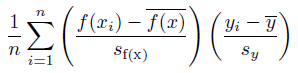
Where sf(x) and sy are the uncorrected sample standard deviations of the model and target variable.
How it's used: to maximize normalized covariance. A commonly used error metric for feature exploration, to find patterns that explain the shape of the data. It's faster to optimize than other metrics because it does not require models to discover the scale and offset of the data.
Considerations:
- It ignores the magnitude and the offset of errors. This means that a model optimized for correlation coefficient alone will try to fit the same shape as the target variable, however actual predicted values may not be close to the actual values.
- It is always on a [-1, 1] scale regardless of the scale of your data.
- 1 is a perfect positive correlation, 0 is no correlation, and -1 is a perfect inverse correlation.
Maximum Absolute
The value of the largest absolute error. Smaller values are better.
Details: Maximum Absolute Error is computed as:
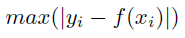
How it's used: to minimize the largest error. It is used when you only care about the single highest error, and when you are looking for an exact fit, such as symbolic simplification. It would typically be used when there is no noise in the data (e.g., processed, simulated, or generated data).
Considerations:
- The whole model's evaluation depends on a single data point.
- It is best when the input data has little to no noise.
Mean Logarithm Squared
The mean of the logs of the squared residuals. A smaller value indicates a lower error.
Details: Mean Logarithm Squared Error is computed as:
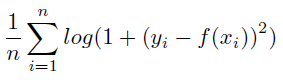
where log is the natural log.
How it's used: to minimize the squashed log error. It decreases the effect of large errors, which can help to decrease the role of outliers in shaping your model.
Considerations:
- It assumes diminishing marginal disutility of error with error size.
Median Absolute
The median of the residual values. A smaller value indicates lower error.
Details: Median Absolute Error is calculated as:
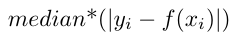
Note
For performance reasons, Eureqa models use an estimated (rather then exact) median value. For small datasets, the estimated median value may differ significantly from the actual value.
How it's used: to minimize the median error value. If you expect your residuals to have a very skewed distribution, it is best at handling high noise and outliers.
Considerations:
- The scale of errors on either side of the median will have no effect.
- It is the most robust error metric to outliers.
- The estimated median may be inaccurate for very small datasets.
Interquartile Mean Absolute
The mean of the absolute error within the interquartile range (the middle 50%) of the residual errors. A smaller value indicates lower error.
Details: The Interquartile Mean Absolute Error is calculated by taking the Mean Absolute Error of the middle 50% of residuals.
How it's used: to minimize the error of the middle 50% error values. It is used when the target variable may contain large outliers, or when you care most about "on average" performance. It is similar to the median error in that it is very robust to outliers.
Considerations:
- It ignores the smallest and largest errors.
AIC Absolute
The Akaike Information Criterion (AIC) based on the Mean Absolute Error. It is a combination of the normalized Mean Absolute Error and a penalty based on the number of model parameters. A lower value indicates a better quality model. Unlike other error metrics, AIC may be a negative value, approaching negative infinity, for increasingly accurate models.
Details: AIC Absolute Error is calculated as:
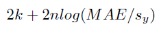
where log is the natural logarithm, sy is the standard deviation of the target variable, MAE is the mean of the absolute value of the residuals:
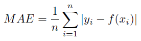
and k is the number of parameters in the model (including terms with a coefficient of 1).
How it's used: to minimize the residual error and number of parameters. It penalizes complexity by including the number of parameters in the loss function. This metric can be useful if you want to directly limit and penalize the number of parameters in a model, for example when modeling physical systems or for other problems where solutions with fewer free parameters are preferred. It is similar to the AIC-Mean Squared Error metric but is more tolerant to outliers.
Considerations:
- Searches using this metric may produce fewer solutions and limit the number of very complex solutions.
- Optimizing for this metric ensures you only get AIC-optimal models.
- Assumes the noise follows a double exponential distribution.
AIC Squared
The Akaike Information Criterion (AIC). It is a combination of the normalized Mean Squared Error and a penalty based on the number of model parameters. A lower value indicates a better quality model. Unlike other error metrics, the value may be negative, approaching negative infinity, for increasingly accurate models.
Details: AIC Squared Error is calculated as:
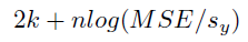
where log is the natural logarithm, sy is the standard deviation of the target variable, MSE is the mean of the squared value of the residuals:
and k is the number of parameters in the model (including terms with a coefficient of 1).
How it's used: to minimize the squared residual error and number of parameters. It penalizes complexity by including number of parameters in the loss function. This metric can be useful if you want to directly limit and penalize the number of parameters in a model, for example when modeling physical systems or for other problems where solutions with fewer free parameters are preferred.
Considerations:
- Searches using this metric may produce fewer solutions and limit the number of very complex solutions.
- Optimizing for this metric ensures you only get AIC-optimal models.
- It assumes the residuals have a normal distribution.
Rank Correlation (Rank-r)
The Correlation Coefficient between the ranks of the predicted values and the actual values. A higher value indicates a stronger positive correlation, with 0 representing no correlation and 1 representing a perfect rank correlation.
Details: The rank correlation is calculated as the correlation coefficient between the ranks of predicted values and ranks of actual values, meanings it optimizes models whose outputs can be used for ranking things. Ranks are computed by sorting each in ascending order and assigning incrementing values to each row based on its sorted position.
How it's used: to maximize the correlation between predicted and actual rank. Use for problems where it is important that a model be able to predict a relative ordering between points, but where the actual predicted values are not important.
Considerations:
- The variables must be ordinal, interval, or ratio.
- A rank correlation of 1 indicates that there is a monotonic relationship between the two variables.
- It is always on a [-1,1] scale, regardless of the scale of your data.
- If ranges for the actual and prediction values are vastly different, the resulting plots may not appear to display as expected. For example, prediction values of (29, 30, 32, 584, 9999, 10000) - or even (100001, 100002, 100003, 100004, 100005, 100006) - and actual values of (1, 2, 3, 4, 5, 6) have the same rank order of the predictions and actuals and so will result in a zero error. But, because the range of predictions vary wildly, they may not be visible on a plot of the actuals.
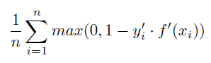
Hinge Loss
The mean “hinge loss” for classification predictions. Hinge loss increasingly penalizes wrong predictions as they get more confident but treats true predictions identically after they reach a minimum threshold value. A smaller value indicates lower error.
Details: Hinge Loss Error is computed as:
where, for this metric, binary classes typically represented as 0 and 1 are re-scaled to be -1 and 1 respectively:
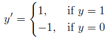
and
With this calculation, when the prediction f(xi) and actual yi have the same sign (a correct prediction) and the predicted value >= 1, the error is considered 0, while when they have a different sign (an incorrect prediction), the error increases linearly with f(xi).
How it's used: to minimize classification error. Hinge Loss Error is a one-sided metric that increasingly penalizes wrong predictions as they get more confident, but treats all true predictions identically after they reach a minimum threshold value.
Considerations:
- When using for classification problems, the target expression should not include the logistic() function. This error metric expects that predicted values will have a larger range.
- It assumes a threshold value of 0.5 when turning a predicted score into a 0 or 1 prediction.
Slope Absolute
The mean absolute error of the predicted row-to-row deltas and the actual row-to-row deltas. A smaller value indicates a lower error.
Details: Slope Absolute Error is computed as:
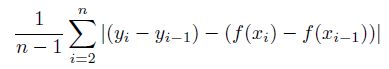
For each side of the model equation (predicted values and actual values), this metric computes row-to-row "deltas" between the value of each row and its previous row. The Slope Absolute Error is the Mean Absolute Error between the actual deltas and the predicted deltas.
How it's used: to minimize the error of the deltas. It is used for time series analysis where you are trying to predict the change from one time period to the next.
Considerations:
- It is an experimental (non-standard) error metric.
- It fits the shape of a dataset; actual predicted values may not be in the same range as the actual values.