Time series framework
This section describes the basic time series framework, window-created gaps, and common data patterns for time series problems.
Basic time series framework
The simple time series modeling framework can be illustrated as follows:
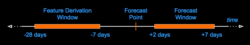
- The Forecast Point defines an arbitrary point in time for making a prediction.
- The Feature Derivation Window (FDW), to the left of the Forecast Point, defines a rolling window of data that DataRobot uses to derive new features for the modeling dataset.
- Finally, the Forecast Window (FW), to the right of the Forecast Point, defines the range of future values you want to predict (known as the Forecast Distances (FDs)). The Forecast Window tells DataRobot, "Make a prediction for each day inside this window."
Note that the values specified for the Forecast Window are inclusive. For example, if set to +2 days through +7 days, the window includes days 2, 3, 4, 5, 6, and 7. By contrast, the Feature Derivation Window does not include the left boundary but does include the right boundary. (In the image above, DataRobot uses from 7 days before the Forecast Point to 27 days before, but not day 28). This is important to consider when setting the window because it means that DataRobot sets lags exclusive of the left (older) side, but inclusive of the right (newer) side. Be aware that when using a differenced feature list at prediction time, you need to account for the difference. For example, if a model uses 7-day differencing, and the feature derivation window spanned [-28 to 0] days, the effective derivation window would be [-35 to 0] days.
The time series framework captures the business logic of how your model will be used by encoding the amount of recent history required to make new predictions. Setting the recent history configures a rolling window used for creating features, the forecast point, and ultimately, predictions. In other words, it sets a minimum constraint on the feature creation process and a minimum history requirement for making predictions.
In the framework illustrated above, for example, DataRobot uses data from the previous 28 days and as recent as up to 7 days ago. The forecast distances the model will report are for days 2 through 7—your predictions will include one row for each of those days. The Forecast Window provides an objective way to measure the total accuracy of the model for training, where total error can be measured by averaging across all potential Forecast Points in the data and the accuracy for each forecast distance in the window.
Window-created gaps
Now, add the gaps that are inherent to time series problems.

This illustration includes the "blind history" (1) and "can't operationalize" (2) periods.
“Blind history" captures the gap created by the delay of access to recent data (e.g., “most recent” may always be one week old). It is defined as the period of time between the smaller of the values supplied in the Feature Derivation Window and the Forecast Window. A gap of zero means "use data up to, and including, today;" a gap of one means "use data starting from yesterday" and so on.
The "can't operationalize" period defines the gap of time immediately after the Forecast Point and extending to the beginning of the Forecast Window. It represents the time required once a model is trained, deployed to production, and starts making predictions—the period of time that is too near-term to be useful. For example, predicting staffing needs for tomorrow may be too late to allow for taking action on that prediction.
Common patterns of time series data
Time series models are built based on consideration of common patterns in time series data:
-
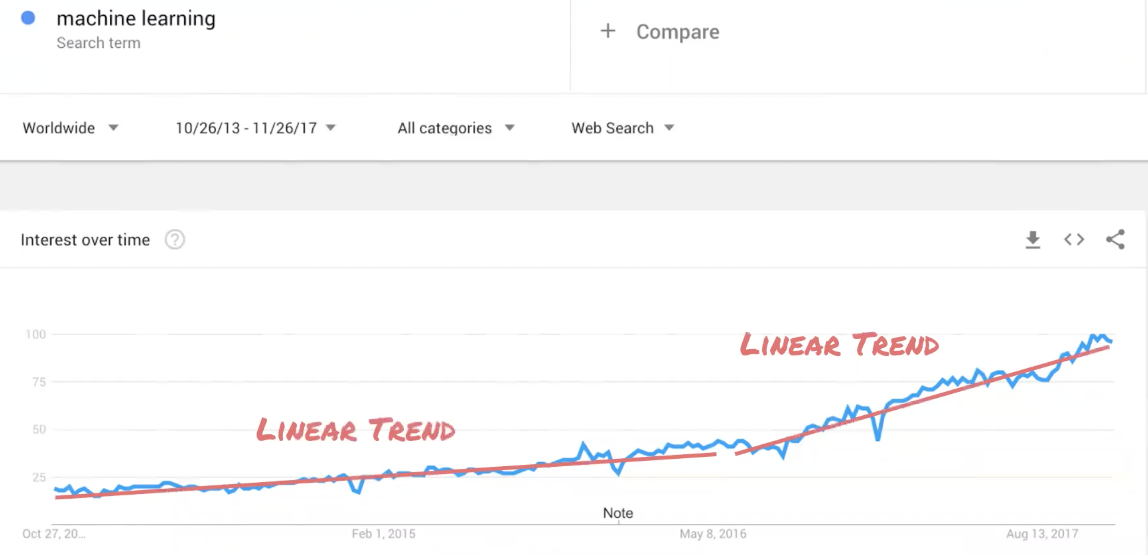
Linearity : A specific type of trend. Searching on the term "machine learning," you see an increase over time. The following shows the linear trends (you can also view as a non-linear trend) created by the search term, showing that interest may fluctuate but is growing over time:
-
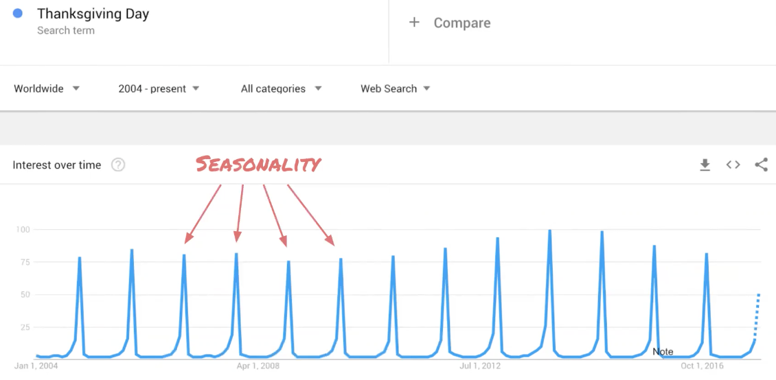
Seasonality: Searching on the term "Thanksgiving" shows periodicity. In other words, spikes and dips are closely related to calendar events (for example, each year starting to grow in July, falling in late November):
-
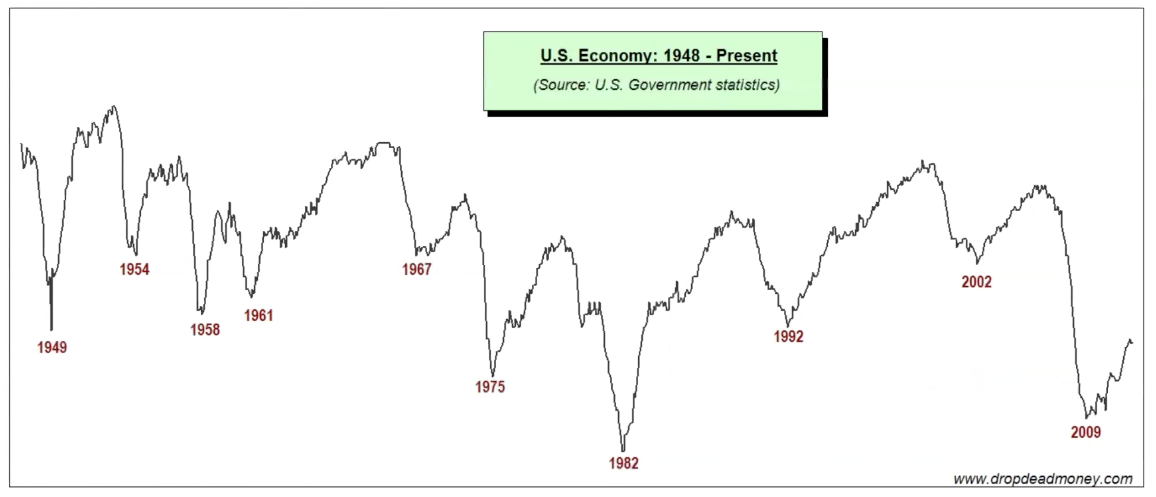
Cycles: Cycles are similar to seasonality, except that they do not necessarily have a fixed period and are generally require a minimum of four years of data to be qualified as such. Usually related to global macroeconoimc events or changes in the political landscapes, cycles can be seen as a series of expansions and recessions:
-
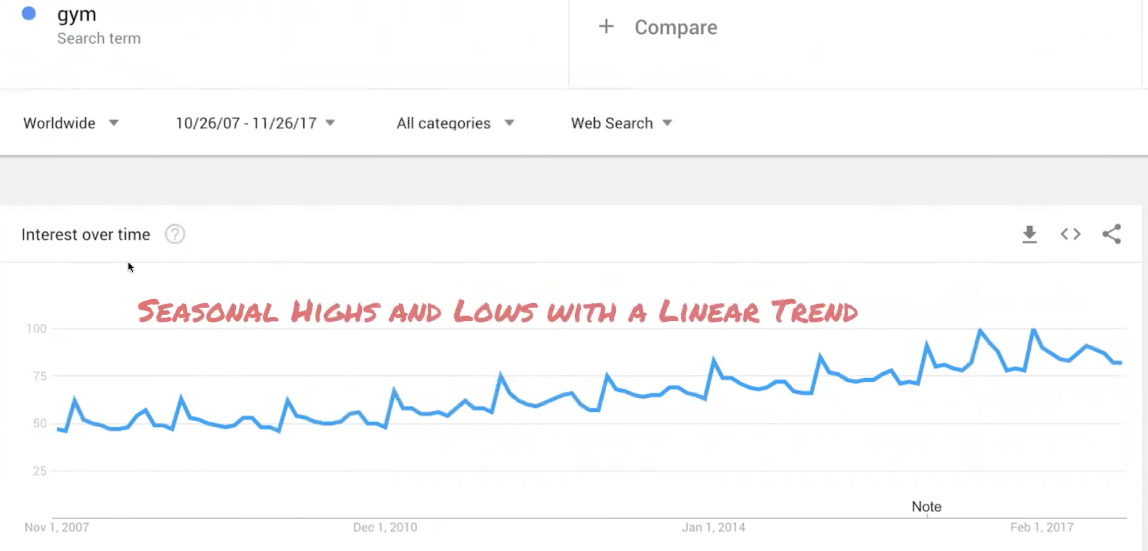
Combinations: Data can combine patterns as well. Consider searching the term "gym." Search interest spikes every January with lows over the holidays. Interest, however, increases over time. In this example you can see both seasonality with linear a trend: