Create experiments
There are two AI experimentation "types" available in Workbench:
-
Time-aware modeling, described on this page, models using time-relevant data to make row-by-row predictions, time series forecasts, or current value predictions "nowcasts".
-
Predictive modeling, makes row-by-row predictions based on your data (see basic and advanced settings).
Note
There is extensive material available about the fundamentals of time aware modeling. While the instructions largely represent the workflow as applied in DataRobot Classic, the reference material describing the framework, feature derivation process, and more are still applicable.
Experiments are the individual "projects" within a Use Case. They allow you to vary data, targets, and modeling settings to find the optimal models to solve your business problem. Within each experiment, you have access to its Leaderboard and model insights, as well as experiment summary information.
Preview
Time series modeling is on by default.
Feature flag: Enable Workbench for Time Series Projects
Create basic
Follow the steps below to create a new experiment from within a Use Case.
Note
You can also start modeling directly from a dataset by clicking the Start modeling button. The Set up new experiment page opens. From there, the instructions follow the flow described below.
Create a feature list
Before modeling, you can create a custom feature list from the Data tab. If you select that list during modeling setup, DataRobot creates the modeling data using only the features in that list.
To create a new list:
- From the Use Case, select the dataset you plan to model with to open the data preview.
-
Click the dropdown at the top of the page and select + New feature list to open the Features view.
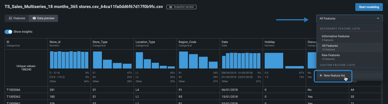
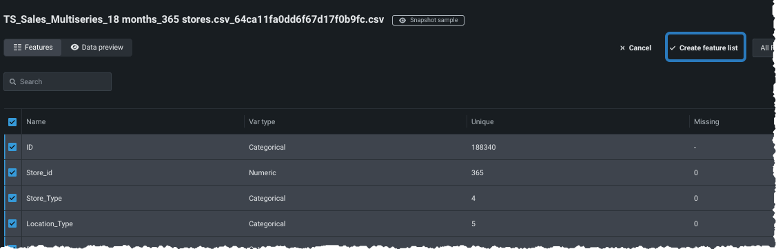
-
Select the checkbox next to each feature you want to include in your custom list. Then, click Create feature list, enter a name and description (optional), and click Save changes.
DataRobot automatically creates new feature lists after the feature derivation process. Once modeling completes, you can train new models using the time-aware lists. Learn more about feature lists and the data tab here.
Add experiment
From within a Use Case, click Add and select Experiment. The Set up new experiment page opens, which lists all data previously loaded to the Use Case.

Add data
Add data to the experiment, either by adding new data (1) or selecting a dataset that has already been loaded to the Use Case (2).
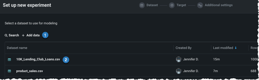
Once the data is loaded to the Use Case (option 2 above), click to select the dataset you want to use in the experiment. Workbench opens a preview of the data.
From here, you can:
| Option | |
|---|---|
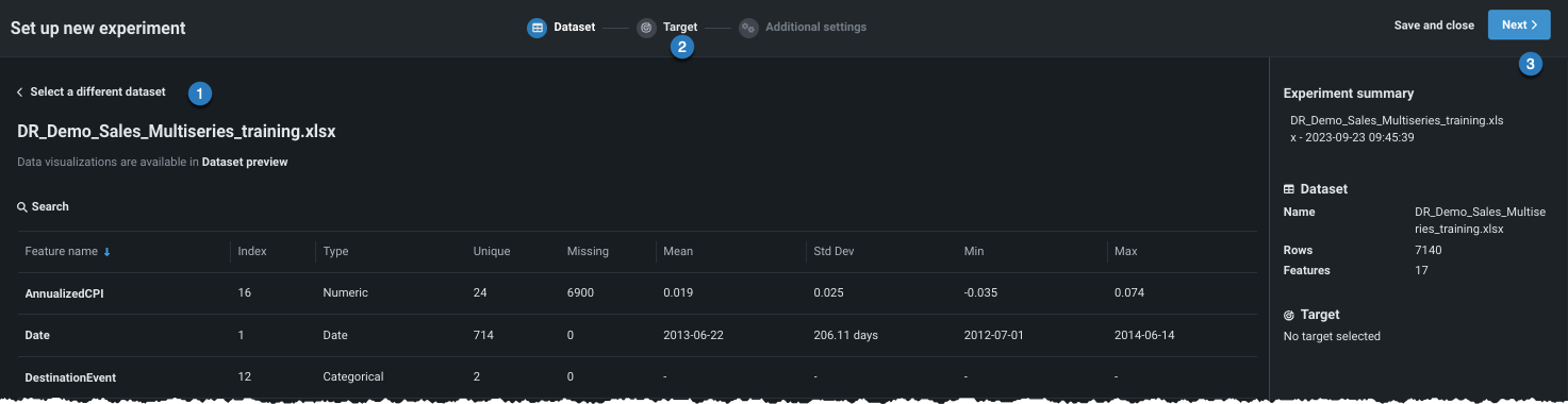
| 1 | Click to return to the data listing and choose a different dataset. |
| 2 | Click the icon to proceed and set the target. |
| 3 | Click Next to proceed and set the target. |
Set target
Once you have proceeded to target selection, Workbench prepares the dataset for modeling (EDA 1).
Note
From this point forward in experiment creation, you can either continue setting up your experiment (Next) or you can exit. If you choose Exit, you are prompted discard changes or to save all progress as a draft. In either case, on exit you are returned to the point where you began experiment setup and EDA1 processing is lost. If you chose Exit and save draft, the draft is available in the Use Case directory.
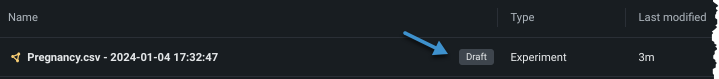
If you open a Workbench draft in DataRobot Classic and make changes that introduce features not supported in Workbench, the draft will be listed in your Use Case but will not be accessible except through the classic interface.
When EDA1 finishes, to set the target, either:
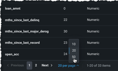
Scroll through the list of features to find your target. If it is not showing, expand the list from the bottom of the display:
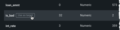
Once located, click the entry in the table to use the feature as the target.
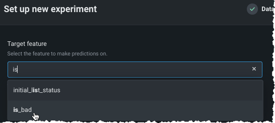
Type the name of the target feature you would like to predict in the entry box. DataRobot lists matching features as you type:
Depending on the number of values for a given target feature, DataRobot automatically determines the experiment type—either regression or classification. Classification experiments can be either binary (binary classification) or more than two classes (multiclass). The following table describes how DataRobot assigns a default problem type for numeric and non-numeric target data types:
| Target data type | Number of unique target values | Default problem type | Use multiclass classification? |
|---|---|---|---|
| Numeric | 2 | Classification | No |
| Numeric | 3+ | Regression | Yes, optional |
| Non-numeric | 2 | Binary classification | No |
| Non-numeric | 3-100 | Classification | Yes, automatic |
| Non-numeric, numeric | 100+ | Aggregated classification | Yes, automatic |
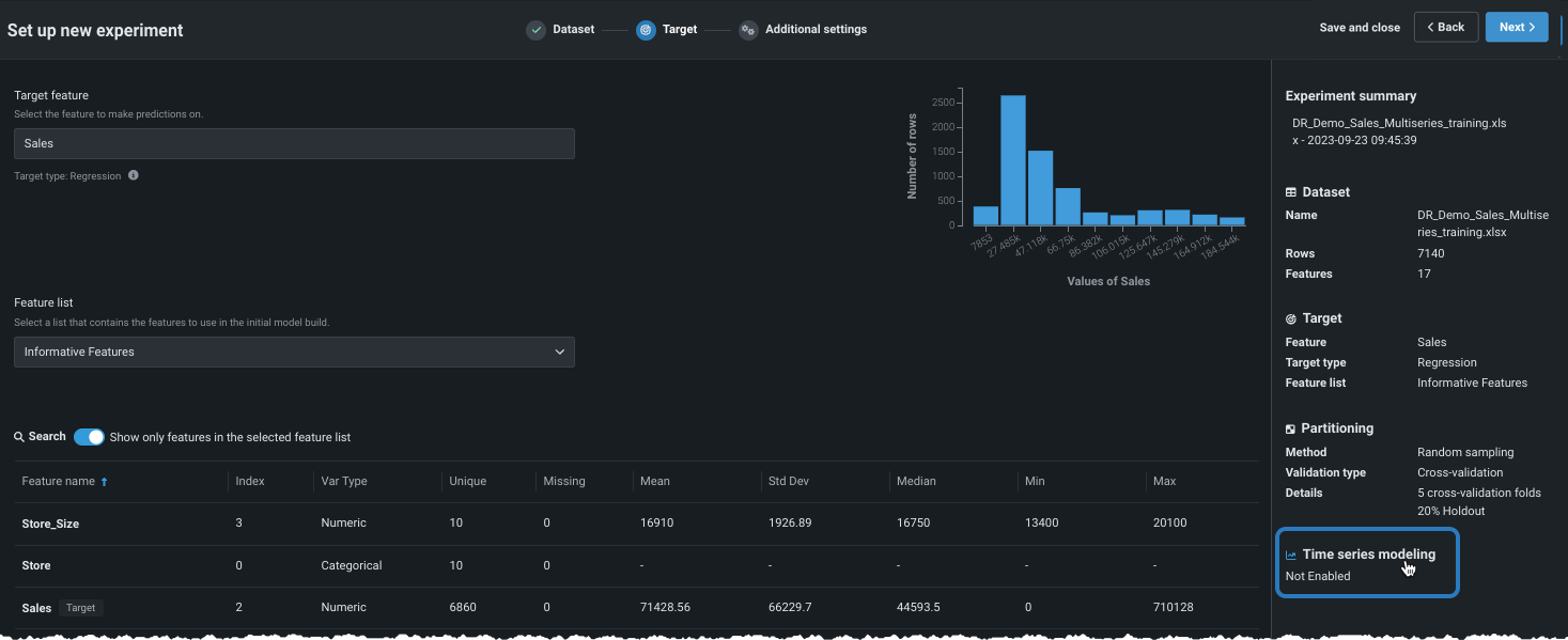
With a target selected, Workbench displays a histogram providing information about the target feature's distribution and, in the right pane, a summary of the experiment settings.

From here you can:
-
Change a regression experiment to a multiclass experiment.
-
Click Next to view Additional settings, where you can build models with the default settings or modify those settings.
-
For multiclass classification experiments, click Show more classification settings to further configure aggregation settings.
If using the default settings, click Start modeling to begin the Quick mode Autopilot modeling process.
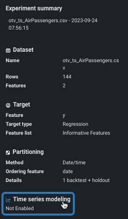
After the target is defined, Workbench displays a histogram providing information about the target feature's distribution and, in the right panel, a summary of the experiment settings. From here, you can build models with the default settings for predictive modeling.
If DataRobot detected a column with time features (variable type "Date") in the dataset, as reported in the Experiment summary, you can build time-aware models.
Customize basic settings
Prior to enabling time-aware modeling, you can change several of the basic modeling settings. These options are common to both predictive and time-aware modeling.
Changing experiment parameters is a good way to iterate on a Use Case. Before starting to model, you can change a variety of settings:
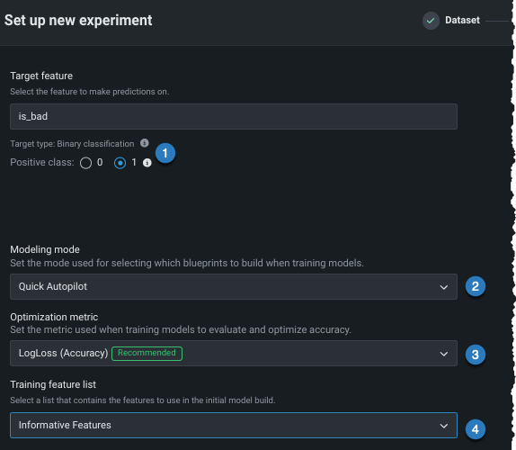
| Setting | To change... | |
|---|---|---|
| Positive class | For binary classification projects only. The class to use when a prediction scores higher than the classification threshold. | |
| Modeling mode | The modeling mode, which influences the blueprints DataRobot chooses to train. | |
| Optimization metric | The optimization metric to one different from DataRobot's recommendation. | |
| Training feature list | The subset of features that DataRobot uses to build models. |
After changing any or all of the settings described, click Next to customize more advanced settings and enable time-aware modeling.
Change modeling mode
By default, DataRobot builds experiments using Quick Autopilot; however, you can change the modeling mode to train specific blueprints or all applicable repository blueprints.
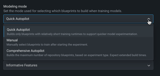
The following table describes each of the modeling modes:
| Modeling mode | Description |
|---|---|
| Quick (default) | Using a sample size of 64%, Quick Autopilot runs a subset of models, based on the specified target feature and performance metric, to provide a base set of models that build and provide insights quickly. |
| Manual | Manual mode gives you full control over which blueprints to execute. After EDA2 completes, DataRobot redirects you to the blueprint repository where you can select one or more blueprints for training. |
Change optimization metric
The optimization metric defines how DataRobot scores your models. After you choose a target feature, DataRobot selects an optimization metric based on the modeling task. Typically, the metric DataRobot chooses for scoring models is the best selection for your experiment. To build models using a different metric, overriding the recommended metric, use the Optimization metric dropdown:
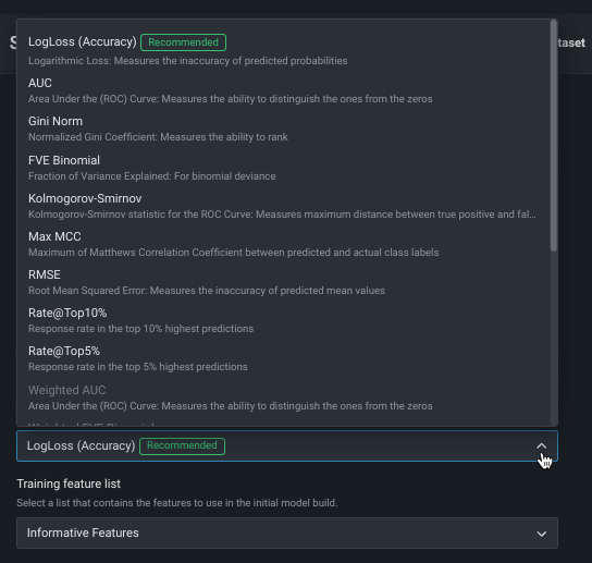
See the reference material for a complete list and descriptions of available metrics.
Change feature list (pre-modeling)
Feature lists control the subset of features that DataRobot uses to build models. Workbench defaults to the Informative Features list, but you can modify that before modeling. To change the feature list, click the Feature list dropdown and select a different list:
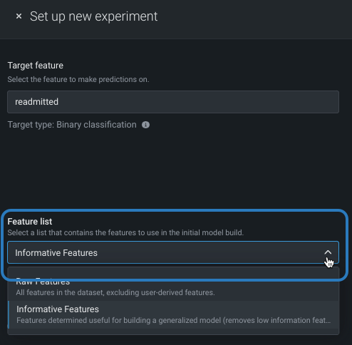
You can also change the selected list on a per-model basis once the experiment finishes building.
Set additional automation
Before moving to advanced settings or beginning modeling, you can configure other automation settings.
After the target is set and the basic settings display, expand Show additional automation settings to see additional options.
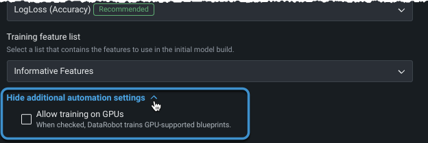
Train on GPUs
Availability information
GPU workers are a premium feature. Contact your DataRobot representative for information on enabling the feature.
For datasets that include text and/or images and require deep learning models, you can select to train on GPUs to speed up training time. While some of these models can be run on CPUs, others require GPUs to achieve reasonable response time. When Allow training on GPUs is selected, DataRobot detects blueprints that contain certain tasks and includes GPU-supported blueprints in the Autopilot run. Both GPU and CPU variants are available in the repository, allowing a choice of which worker type to train on; GPU variant blueprints are optimized to train faster on GPU workers. Notes about working with GPUs:
- Once the Leaderboard populates, you can easily identify GPU-based models using filtering.
- When retraining models, the resulting model is also trained using GPUs.
- When using Manual mode, you can identify GPU-supported blueprints by filtering in the blueprint repository.
- If you did not initially select to train with GPUs, you can add GPU-supported blueprints via the repository or by rerunning modeling.
-
Models trained on GPUs are marked with a badge on the Leaderboard:
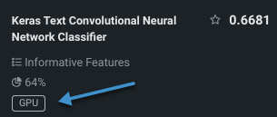
You can also change the selected list on a per-model basis once the experiment finishes building.
Configure additional settings
Choose the Additional settings tab to set more advanced modeling capabilities. Note that the Time series modeling tab will be available or greyed out depending on whether DataRobot found any date/time features in the dataset.
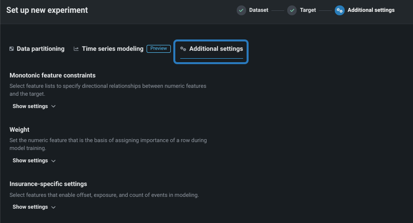
Configure the following, as required by your business use case.
Note
You can complete the time-aware configuration or the additional settings in either order.
Monotonic feature constraints
Monotonic constraints control the influence, both up and down, between variables and the target. In some use cases (typically insurance and banking), you may want to force the directional relationship between a feature and the target (for example, higher home values should always lead to higher home insurance rates). By training with monotonic constraints, you force certain XGBoost models to learn only monotonic (always increasing or always decreasing) relationships between specific features and the target.
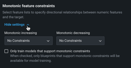
Using the monotonic constraints feature requires creating special feature lists, which are then selected here. Note also that when using Manual mode, available blueprints are marked with a MONO badge to identify supporting models.
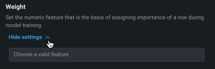
Weight
Weight sets a single feature to use as a differential weight, indicating the relative importance of each row. It is used when building or scoring a model—for computing metrics on the Leaderboard—but not for making predictions on new data. All values for the selected feature must be greater than 0. DataRobot runs validation and ensures the selected feature contains only supported values.
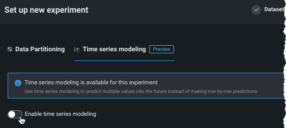
Enable time-aware modeling
Time-aware modeling is based on Date/time as the partitioning method. There are two types of time-aware modeling:
- Simple Date/time partitioning, which assigns rows to backtests chronologically.
- Time series modeling for forecasting multiple future values of the target.
The workflow for both begins with partitioning. If you want forecasts instead of predictions, or want to take advantage of DataRobot's automated time series feature engineering, you will continue setup on the Time series modeling tab.
graph TB
  A(Start time-aware modeling) --> B[Enable date/time partitioning];
  B --> C[Set ordering feature];
  C --> D[Set backtest partitions];
  D --> E[Set sampling];
  E --> F{Predictions or forecasts?} --> | Predictions|G[Start modeling];
  F --> |Forecasts|H[Enable time series modeling]
  H --> I[Continue experiment setup]
  I --> J[Start modeling]
Date and date range representation
DataRobot uses date points to represent dates and date ranges within the data, applying the following principles:
- All date points adhere to ISO 8601, UTC (e.g., 2016-05-12T12:15:02+00:00), an internationally accepted way to represent dates and times, with some small variation in the duration format. Specifically, there is no support for ISO weeks (e.g., P5W).
- Models are trained on data between two ISO dates. DataRobot displays these dates as a date range, but inclusion decisions and all key boundaries are expressed as date points. When you specify a date, DataRobot includes start dates and excludes end dates.
- Once changes are made to formats using the date partitioning column, DataRobot converts all charts, selectors, etc. to this format for the project.
- When changing partition year/month/day settings, the month and year values rebalance to fit the larger class (for example, 24 months becomes two years) when possible. However, because DataRobot cannot account for leap years or days in a month as it relates to your data, it cannot convert days into the larger container.
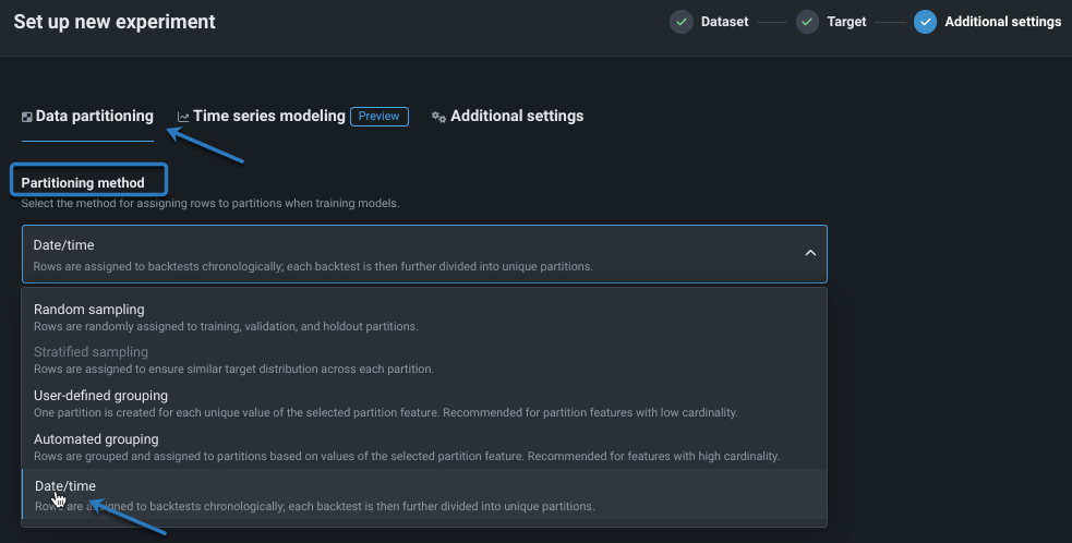
1. Enable date/time partitioning
To enable time-aware modeling, first set the partitioning method to Date/time. To do this do one of the following:
- Open the Data partitioning tab.
- Click on Partitioning in the experiment summary panel, which opens the Data partitioning tab.
From the Data partitioning tab, select Date/time as the partitioning method:
2. Set ordering feature
After setting the partitioning method to date/time, set the ordering feature—the primary date/time feature DataRobot uses for modeling.
Note
All other settings can be changed or left at the default. The Experiment summary, in the right-hand panel, updates as setup continues.
Select the ordering feature. If only one qualifying feature is detected, the field is autofilled. If multiple features are available, click in the box to display a list of all qualifying features. If a feature is not listed, it was not detected as type date and cannot be used.
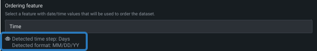
Once set, DataRobot:
-
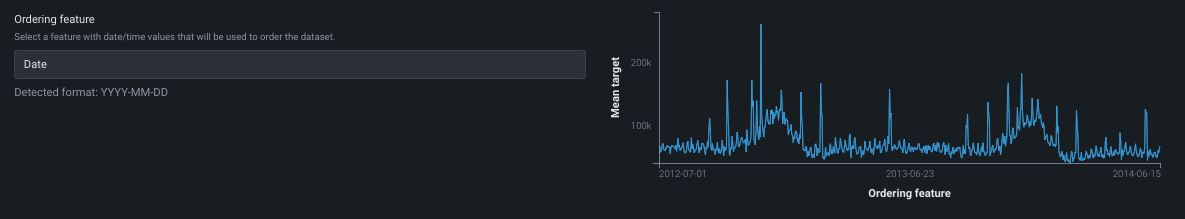
Detects and reports the date and/or time format (standard GLIBC strings) for the selected feature:
-
Computes and then loads a feature-over-time histogram of the ordering feature. Note that if your dataset qualifies for multiseries modeling, this histogram represents the average of the time feature values across all series plotted against the target feature.
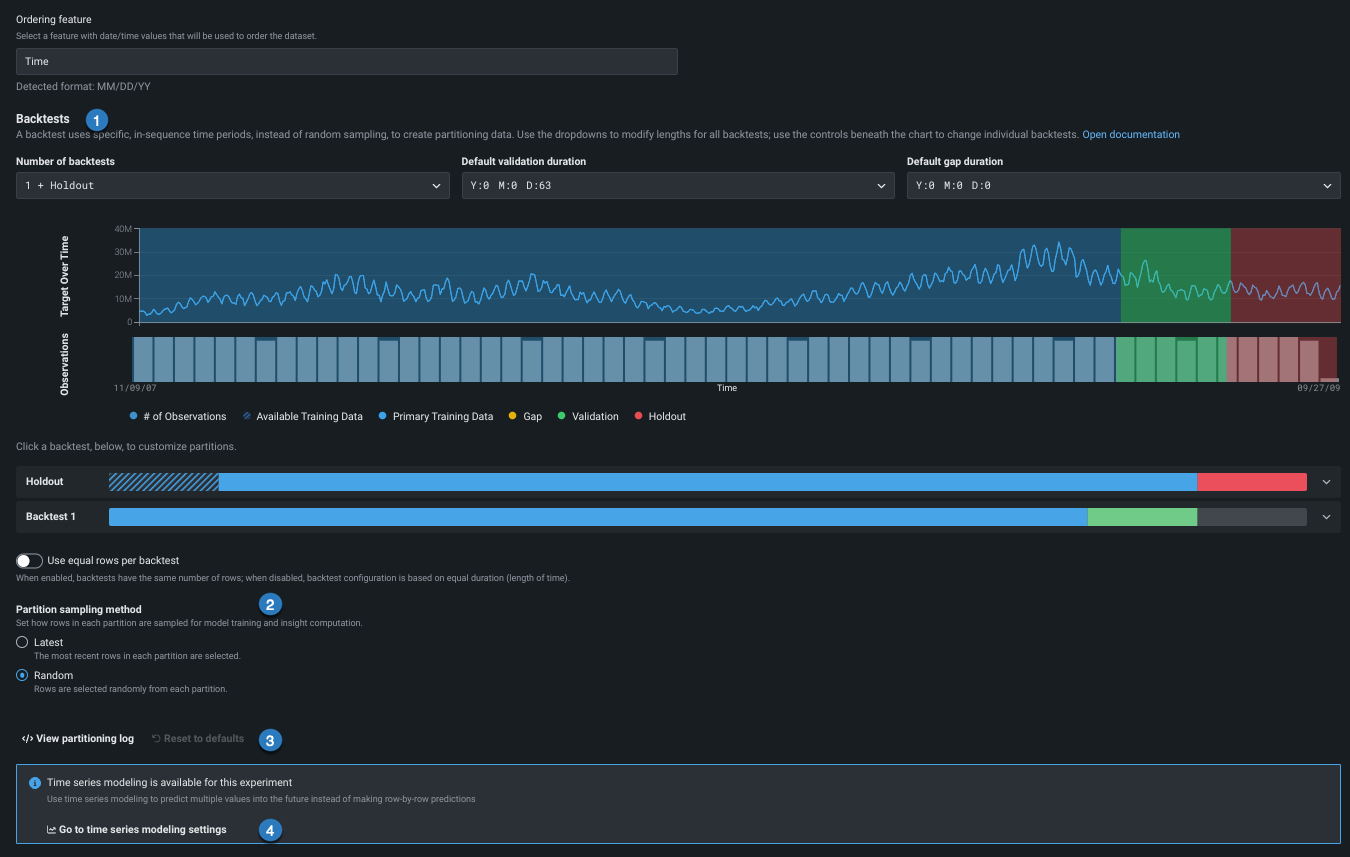
3. Set backtest partitions
Once the ordering feature is set, backtest configuration becomes available. Backtests are the time-aware equivalent of cross-validation, but based on time periods or durations instead of random rows. DataRobot sets defaults based on the characteristics of the dataset and can generally be left as-is—they will result in robust models.
Use the links in the table below to change the default settings:
| Field | Description | |
|---|---|---|
| 1 | Backtests | Sets the number and duration of backtesting partitions. |
| 2 | Row assignment | Sets how rows are assigned to backtests and the sampling method. |
| 3 | Partitioning log / Reset | Provides a downloadable log that reports on partition creation and provides a reset link. |
| 4 | Time series modeling settings | Opens the Time series modelingtab to enable forecasting and access additional options. |
Learn more
The following sections provide detailed explanations of each concept described in this configuration:
Change number of backtests
First, change the number of backtests if desired.
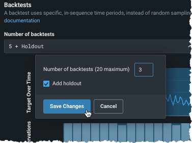
The default number of backtests is dependent on the project parameters, but you can configure up to 20. Before setting the number of backtests, use the histogram to validate that the training and validation sets of each fold will have sufficient data to train a model.
Backtest requirements
- For OTV, backtests require at least 20 rows in each validation and holdout fold and at least 100 rows in each training fold. If you set a number of backtests that results in any of the partitions not meeting those criteria, DataRobot only runs the number of backtests that do meet the minimums (and marks the display with an asterisk).
- For time series, backtests require at least 4 rows in validation and holdout and at least 20 rows in the training fold. If you set a number of backtests that results in any of the partitions not meeting those criteria, the project could fail. See the time series partitioning reference for more information.
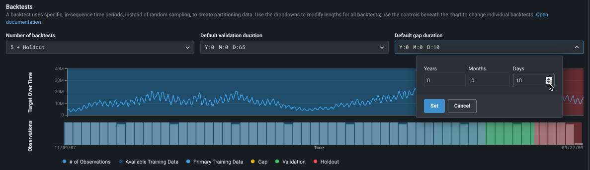
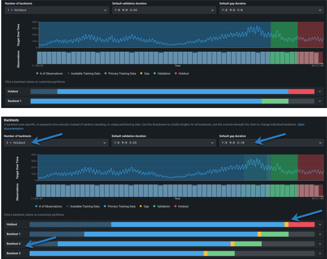
Change partition durations
Next, configure the backtesting partitions. If you don't modify any settings, DataRobot disperses rows to backtests equally. However, you can customize backtest gap, training, validation, and holdout data either:
- To apply globally to all backtests in the experiment, use the dropdowns.
- To apply changes to individual backtests, click the bars below the visualization. Individual settings override global settings. Once you modify settings for an individual backtest, any changes to the global settings are not applied to the edited backtest.
As you add backtests to the experiment configuration, the period of training data used shortens. The validation and gap remain set to the duration set in the dropdowns (unless changed individually per backtest).
Review the default partition settings and click to make changes if needed:
The following provides an overview of the application of each partition, but review the linked material for more detail.
| Partition | Description |
|---|---|
| Default validation duration | Sets the size of the partition used for testing—data that is not part of the training set that is used to evaluate a model’s performance. |
| Default gap duration | Sets spaces in time, representing gaps between model training and model deployment. Initially set to zero, DataRobot does not process a gap in testing. When set, DataRobot excludes the data that falls in the gap from use in training or evaluation of the model. |
Note how the changes are reflected in the testing representation:
Set backtest partitions individually
Regardless of which partition you are setting (training, validation, or gap) elements of the editing screens function the same (holdout is a bit different). To change an individual backtest's duration, first, hover on the color band to see specifics of the specific duration settings:
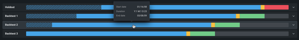
Then, to modify the duration for an individual backtest, click in the backtest to open the inputs:
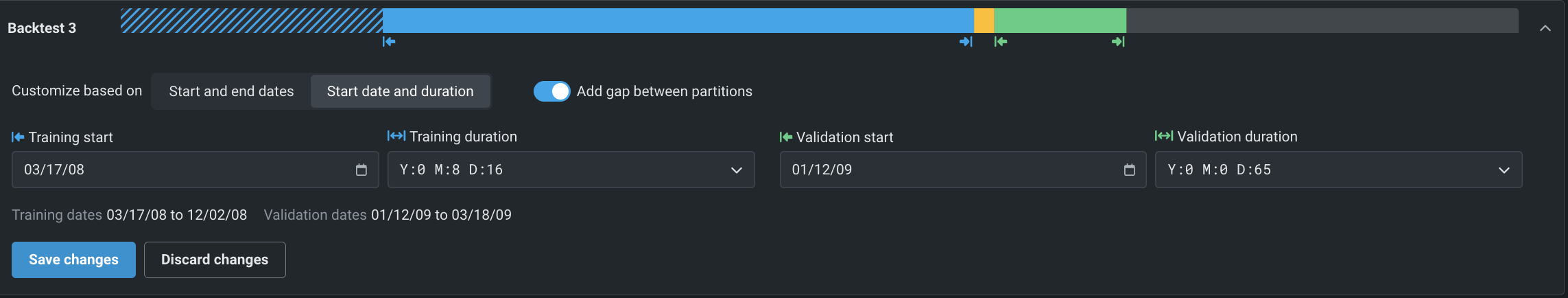
Backtests are based on either start and end dates or start date and duration. Gaps—toggle Add gap between partitions to on to enabled—are derived from the date or duration settings. That is, the gap is created by leaving time steps between the training end and validation start (which, for no gap are the same).
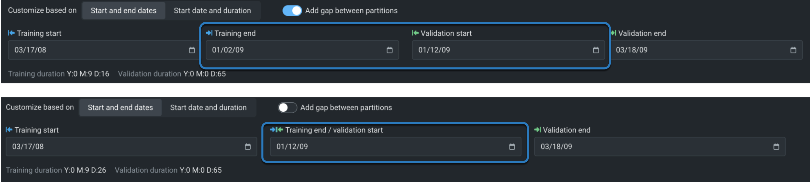
To customize based on start and end dates:
- With a gap, set the start and duration for both training and validation.
- Without a gap, set the training start, training duration, and validation duration.
To customize based on start date and duration:
- With a gap, set the training and validation start and end.
- Without a gap, set the training start, training end, validation start, and validation end.
In all cases, DataRobot verifies entries and reports any required changes:
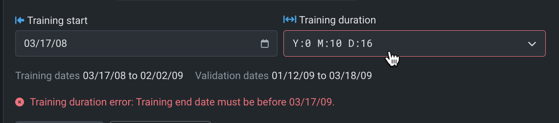
Then, reports valid, set time windows under the input boxes:
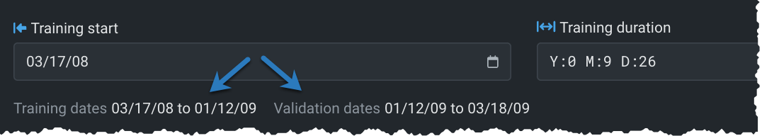
Click Save changes when configuration is complete.
Once you have made changes to a data element, DataRobot adds an EDITED label to the backtest. Use the Reset to defaults link to manually reset durations or number of backtests to the default settings.
Change holdout
By default, DataRobot creates a holdout fold for training models in your project.
Notes on changing holdout
- Generally speaking, although very experiment-dependent, holdout is roughly 10% of the total duration with possible rounding to some "natural" time frame like n weeks, n months. (This is dependent on whether it is simple time-aware or time series.) View the partitioning log for a description of DataRobot's calculations.
- You can only set holdout in the holdout backtest, you cannot change the training data size in that backtest. DataRobot automatically configures the training partition of the holdout backtest.
- If, during the initial partitioning detection, the backtest configuration of the ordering (date/time) feature, series ID, or target results in insufficient rows to cover both validation and holdout, DataRobot automatically disables holdout. If other partitioning settings are changed (validation or gap duration, start/end dates, etc.), holdout is not affected unless manually disabled.
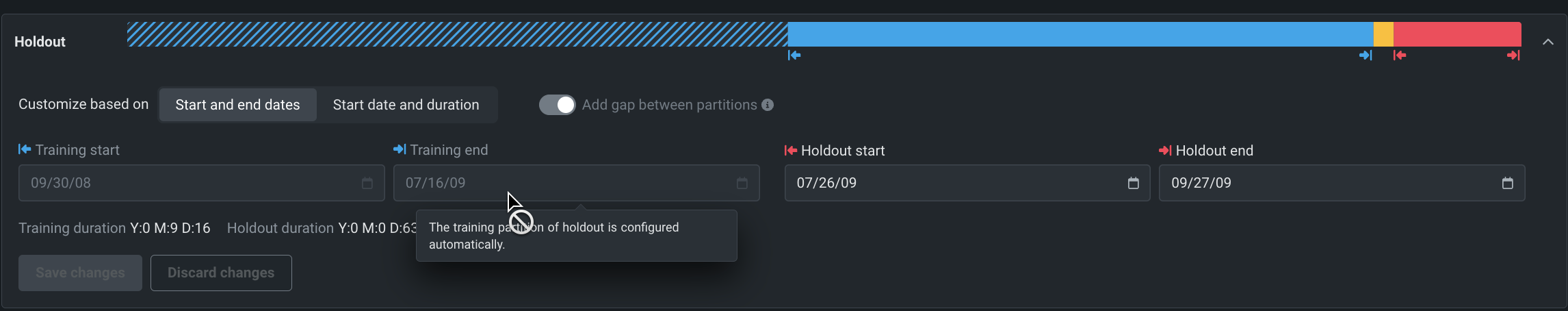
To modify the holdout length, click the holdout backtest to open the inputs and enter new values:
- To customize based on start and end dates, enter holdout start and end dates.
- To customize based on start date and duration enter holdout start and duration.
Note that the training time span and gap settings are configured automatically and cannot be changed on the holdout backtest:
Note
In some cases, however, you may want to create a project without a holdout set. To do so, uncheck the Add holdout box. Any insights that provide an option to switch between validation and holdout will not show the holdout option.
4. Set sampling
After completing backtests, set the row assignment and sampling method.
Row assignment
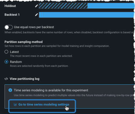
By default, DataRobot ensures that each backtest has the same duration, either the default or the values set from the dropdown(s) or via the bars in the visualization. If you want the backtest to use the same number of rows, instead of the same length of time, use the Equal rows per backtest toggle:
Note
Time series projects also have an option to set row assignment (number of rows or duration) for the training data that is used during feature engineering. Configure this setting in the training window format section.
-
When Equal rows per backtest is checked (which sets the partitions to row-based assignment), only the training end date is applicable.
-
For time series experiments, when Equal rows per backtest is checked, the dates displayed are informative only (that is, they are approximate) and they include padding that is set by the feature derivation and forecast point windows.
Sampling method
Once you have selected the mechanism/mode for assigning data to backtests, select the sampling method, either Random or Latest, to set how to assign rows from the dataset.
Setting the sampling method is particularly useful if a dataset is not distributed equally over time. For example, if data is skewed to the most recent date, the results of using 50% of random rows versus 50% of the latest will be quite different. By selecting the data more precisely, you have more control over the data that DataRobot trains on.
Reset defaults
When you make and save changes to any of the backtest settings, the backtest is marked with a badge (EDITED). Use the Reset to defaults link to manually reset durations or number of backtests to the default settings. Note that for time series experiments, this action does not reset any window settings.
Predictions or forecasts?
For predictive modeling, when you're satisfied with the modeling settings, click Start modeling to begin the Quick mode Autopilot modeling process.
For forecasting, if your experiment is eligible click Go to time series modeling settings to open the Time series modeling tab and continue the configuration.
5. Continue time series configuration
Time series modeling provides an additional set of options, such as identifying series IDs (as applicable), initiating the creation of a derived feature set for modeling, and other particulars of forecasting.
To create experiments that launch time-aware modeling, you can select:
-
Go to time series modeling settings from the Date/time partitioning setup page for time relevant data.
-
Time series modeling in the Experiment summary panel.
Either option opens the settings to the Time series modeling tab. Settings are inherited from the Data partitioning tab (ordering feature and backtests). See and complete, as needed:
The following additional settings are available to configure your time series experiment:
- Select an ordering feature
- Set the series ID (for multiseries projects)
- Customize window settings
- Set additional optional features
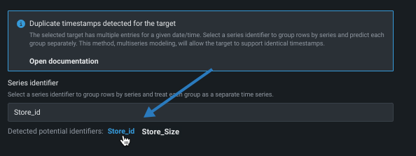
Set series ID
If duplicate time stamps are detected in the data, DataRobot provides options for configuring multiseries modeling. Multiseries modeling allows you to model datasets that contain duplicate timestamps by handling them as multiple, individual time-series datasets. Select a series identifier to indicate which series each row belongs to.
Customize window settings
DataRobot provides default window settings, the Feature Derivation Window (FDW) and Forecast Window (FW), based on the characteristics of the dataset. These settings determine how DataRobot derives features for the modeling dataset by defining the basic framework used for the feature derivation process. They can generally be left as-is.
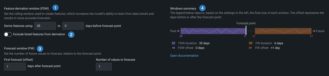
The table below briefly describes the elements of the window setting section of the screen:
Important
If you do decide to modify these values, see the detailed guidance for the meaning and implication of each window.
| Option | Description | |
|---|---|---|
| 1 | Feature Derivation Window (FDW) | Configures the periods of data that DataRobot uses to derive features for the modeling dataset. |
| 2 | Exclude listed features from derivation | Excludes specified features from automated time-based feature engineering (for example, if you have extracted your own time-oriented features and do not want further derivation performed on them). Toggle the option on and select features from the dropdown. |
| 3 | Forecast Window | Sets the time range of forecasts that the model outputs after the forecast point. |
| 4 | Windows summary | Provides a graphical representation of the window settings. Any changes to window values are immediately reflected in the visual. |
Set additional optional features
Two additional optional experiment settings are available:
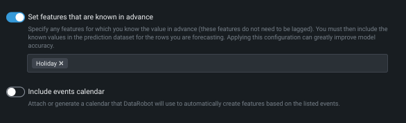
Use Set features that are known in advance to exclude features for which you know their value at modeling time. When a feature is identified with this option, DataRobot will not create lags when deriving modeling data. By informing DataRobot that some variables are known in advance and providing them at prediction time, forecast accuracy is significantly improved. If a feature is flagged as known, however, you must provide its future value at prediction time or predictions will fail. To use this option, toggle it on and select features from the dropdown.
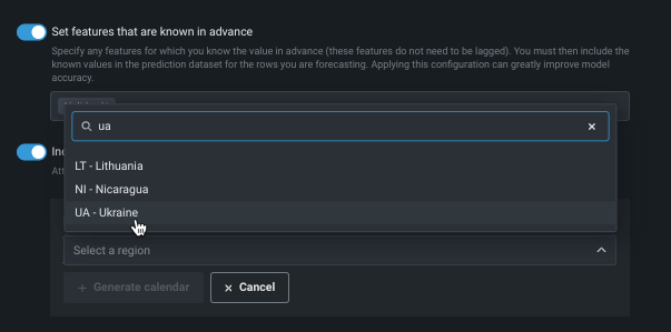
Use Include events calendar to upload or generate an event file that specifies dates or events that require additional attention. DataRobot will use the file to automatically create features based on the listed events. You can choose a local file or one stored in the data registry. Or, click Generate calendar to let DataRobot generate a file of events based on a selected region.
6. Start forecast modeling
After you are satisfied with the modeling settings (which are summarized in the Experiment summary), click Start modeling. When the process begins, DataRobot analyzes the target and creates time-based features to use for modeling. You can control the number of workers applied to the experiment from the queue in the right panel. Increase or decrease workers for your experiment as needed.
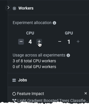
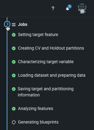
From there, you can also view the jobs that are running, queued, and failed. Expand the queue, if necessary, to see the running jobs and assigned workers.
What's next?
After you start modeling, DataRobot populates the Leaderboard with models as they complete. You can:
- Begin model evaluation on any available model.
- Use the View experiment info option to view a variety of information about the model.
- Display derived modeling data, which is the data that was used to build the model.
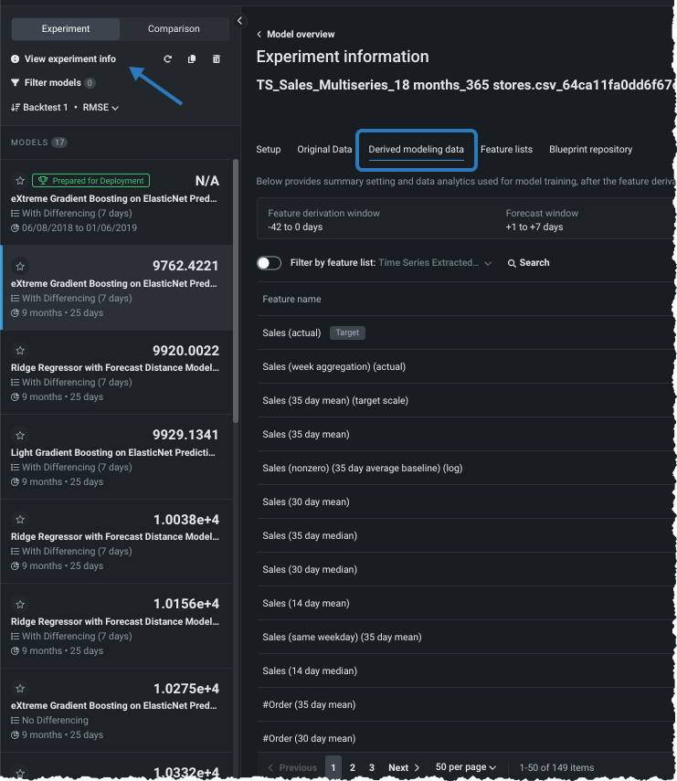
See the following sections for more information on derived modeling data: