Unsupervised predictive modeling
Unsupervised learning uses unlabeled data to surface insights about patterns in your data. Supervised learning, by contrast, uses the other features of your dataset to make predictions. The unsupervised learning setup is described below.
Create basic
Follow the steps below to create a new experiment from within a Use Case.
Note
You can also start modeling directly from a dataset by clicking the Start modeling button. The Set up new experiment page opens. From there, the instructions follow the flow described below.
Create a feature list
Before modeling, you can create a custom feature list from the data explore page. You can then select that list during modeling setup to create the modeling data using only the features in that list. Learn more about feature lists post-modeling here.
Add experiment
From within a Use Case, click Add and select Experiment. The Set up new experiment page opens, which lists all data previously loaded to the Use Case.

Add data
Add data to the experiment, either by adding new data (1) or selecting a dataset that has already been loaded to the Use Case (2).

Once the data is loaded to the Use Case (option 2 above), click to select the dataset you want to use in the experiment. Workbench opens a preview of the data.

From here, you can:
| Option | |
|---|---|
| 1 | Click to return to the data listing and choose a different dataset. |
| 2 | Click the icon to proceed and set the learning type and target. |
| 3 | Click Next to proceed and set the learning type and target. |
Start modeling setup
Once you have proceeded, Workbench prepares the dataset for modeling (EDA 1).
Note
From this point forward in experiment creation, you can either continue setting up your experiment (Next) or you can exit. If you click Exit, you are prompted to discard changes or to save all progress as a draft. In either case, on exit you are returned to the point where you began experiment setup and EDA1 processing is lost. If you chose Exit and save draft, the draft is available in the Use Case directory.

If you open a Workbench draft in DataRobot Classic and make changes that introduce features not supported in Workbench, the draft will be listed in your Use Case but will not be accessible except through the classic interface.
Set learning type
Typically DataRobot works with labeled data, using supervised learning methods for model building. With supervised learning, you specify a target and DataRobot builds models using the other features of your dataset to make predictions.
In unsupervised learning, no target is specified and the data is unlabeled. Instead of generating predictions, unsupervised learning surfaces insights about patterns in your data, answering questions like "Are there anomalies in my data?" and "Are there natural clusters?"
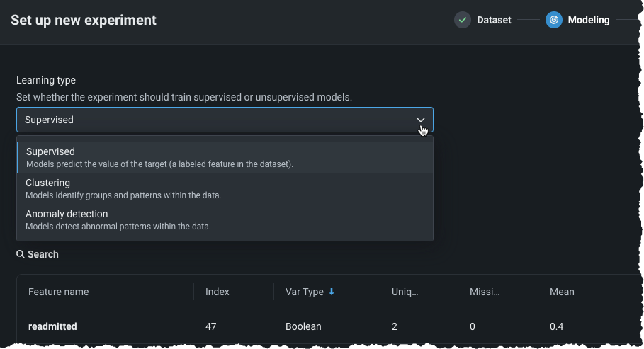
To create an unsupervised learning experiment after EDA1 completes, from the Learning type dropdown, choose one of:
| Learning type | Description |
|---|---|
| Supervised | Builds models using the other features of your dataset to make predictions; this is the default learning type. |
| Clustering (unsupervised) | Using no target and unlabeled data, builds models that group similar data and identify segments. |
| Anomaly detection (unsupervised) | Using no target and unlabeled data, builds that detect abnormalities in the dataset. |

See the feature considerations for things to know when working with unsupervised modeling.
Clustering
Clustering lets you explore your data by grouping and identifying natural segments from many types of data—numeric, categorical, text, image, and geospatial data—independently or combined. In clustering mode, DataRobot captures a latent behavior that's not explicitly captured by a column in the dataset. It is useful when data doesn't come with explicit labels and you have to determine what they should be. Examples of clustering include:
-
Detecting topics, types, taxonomies, and languages in a text collection. You can apply clustering to datasets containing a mix of text features and other feature types or a single text feature for topic modeling.
-
Segmenting a customer base before running a predictive marketing campaign. Identify key groups of customers and send different messages to each group.
-
Capturing latent categories in an image collection.
Configure clustering
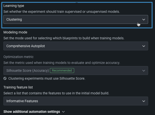
To set up a clustering experiment, set the Learning type to Clustering. Because unsupervised experiments do not specify a target, the Target feature field is removed and the other basic settings become available.

The table below describes each field:
| Field | Description |
|---|---|
| Modeling mode | The modeling mode, which influences the blueprints DataRobot chooses to train. Comprehensive Autopilot, the default, runs all repository blueprints on the maximum Autopilot sample size to provide the most accurate similarity groupings. |
| Optimization metric | Defines how DataRobot scores clustering models. For clustering experiments, Silhouette score is the only supported metric. |
| Training feature list | Defines the subset of features that DataRobot uses to build models. |
Set the number of clusters
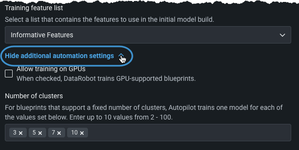
DataRobot trains multiple models, one for each algorithm that supports setting a fixed number of clusters (such as K-Means or Gaussian Mixture Model). The number trained is based on what is specified in Number of clusters, with default values based on the number of rows in the dataset.

For example, if the numbers are set as in the image above, DataRobot runs clustering algorithms using 3, 5, 7, 10 clusters.
To customize the number of clusters that DataRobot trains, expand Show additional automation settings and enter values within the provided range.
When settings are complete, click Next and Start modeling.
Anomaly detection
Anomaly detection, also referred to as outlier or novelty detection, is an application of unsupervised learning. It can be used, for example, in cases where there are thousands of normal transactions with a low percentage of abnormalities, such as network and cyber security, insurance fraud, or credit card fraud. Although supervised methods are very successful at predicting these abnormal, minority cases, it can be expensive and very time-consuming to label the relevant data. See the feature considerations for important information about working with anomaly detection.
Configure anomaly detection
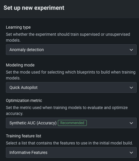
To set up an anomaly detection experiment, set the Learning type to Anomaly detection. No target feature is required.

| Field | Description |
|---|---|
| Modeling mode | The modeling mode, which influences the blueprints DataRobot chooses to train. Quick Autopilot, the default, provide a base set of models that build and provide insights quickly. |
| Optimization metric | Defines how DataRobot scores clustering models. For anomaly detection experiments, Synthetic AUC is the default, and recommended, metric. |
| Training feature list | Defines the subset of features that DataRobot uses to build models. |
When settings are complete, click Next and Start modeling.
Unsupervised insights
After you start modeling, DataRobot populates the Leaderboard with models as they complete. The following table describes the insights available for unsupervised anomaly detection (AD) and clustering for predictive experiments.
| Insight | Anomaly detection | Clustering |
|---|---|---|
| Blueprint | Y | Y |
| Feature Effects | Y | Y |
| Feature Impact | Y | Y |
| Prediction Explanations* | Y | N |
| Cluster Insights** | N | Y |
* XEMP only and Classic only
** Time-aware only
Feature considerations
Unsupervised learning availability is license-dependent:
| Feature | Predictive | Date/time partitioned | Time series |
|---|---|---|---|
| Anomaly detection | Generally available | Generally available | Premium (time series license) |
| Clustering | Premium (Clustering license) | Not available | Premium (time series license) |
Clustering considerations
When using clustering, consider the following:
- Datasets for clustering projects must be less than 5GB.
-
The following is not supported:
- Relational data (summarized categorical features, for example)
- Word Clouds
- Feature Discovery projects
- Prediction Explanations
- Scoring Code
- Composable ML
-
Clustering models can be deployed to dedicated prediction servers, but Portable Prediction Servers (PPS) and monitoring agents are not supported.
- The maximum number of clusters is 100.
Anomaly detection considerations
Consider the following when working with anomaly detection projects:
-
In the case of numeric missing values, DataRobot supplies the imputed median (which, by definition, is non-anomalous).
-
The higher the number of features in a dataset, the longer it takes DataRobot to detect anomalies and the more difficult it is to interpret results. If you have more than 1000 features, be aware that the anomaly score becomes difficult to interpret, making it potentially difficult to identify the root cause of anomalies.
-
If you train an anomaly detection model on greater than 1000 features, Insights in the Understand tab are not available. These include Feature Impact, Feature Effects, Prediction Explanations, Word Cloud, and Document Insights (if applicable).
-
Because anomaly scores are normalized, DataRobot labels some rows as anomalies even if they’re not too far away from normal. For training data, the most anomalous row will have a score of 1. For some models, test data and external data can have anomaly score predictions that are greater than 1 if the row is more anomalous than other rows in the training data.
-
Synthetic AUC is an approximation based on creating synthetic anomalies and inliers from the training data.
-
Synthetic AUC scores are not available for blenders that contain image features.
-
Feature Impact for anomaly detection models trained from DataRobot blueprints is always computed using SHAP. For anomaly detection models from user blueprints, Feature Impact is computed using the permutation-based approach.
-
Because time series anomaly detection is not yet optimized for pure text data anomalies, data must contain some numerical or categorical columns.
-
The following methods are implemented and tunable:
| Method | Details |
|---|---|
| Isolation Forest |
|
| Double Mean Absolute Deviation (MAD) |
|
| One Class Support Vector Machine (SVM) |
|
| Local outlier factor |
|
| Mahalanobis Distance |
|
-
The following is not supported:
-
Projects with weights or offsets, including smart downsampling
-
Scoring Code
-
Anomaly detection does not consider geospatial data (that is, models will build but those data types will not be present in blueprints).
Additionally, for time series projects:
- Millisecond data is the lower limit of data granularity.
- Datasets must be less than 1GB.
- Some blueprints don’t run on purely categorical data.
- Some blueprints are tied to feature lists and expect certain features (e.g., Bollinger Band rolling must be run on a feature list with robust z-score features only).
- For time series projects with periodicity, because applying periodicity affects feature reduction/processing priorities, if there are too many features then seasonal features are also not included in Time Series Extracted and Time Series Informative Features lists.
Additionally, the time series considerations apply.